Welcome to RAPID’s documentation!

This document describes an open source power system simulation toolbox: Resilient Adaptive Parallel sImulator for griD (RAPID), a package of Python codes that implements an advanced power system dynamic simulation framework. RAPID utilizes and incorporates emerging solution techniques; a novel “parallel-in-time” (Parareal) algorithm, adaptive model reduction, and semi-analytical solution methods. Moreover, the whole simulation process for the transmission network has been coupled with OpenDSS, a widely used open-source distribution system simulator, to enable the co-simulation of integrated transmission and distribution systems. RAPID has a great potential to significantly improve the computational performance of time-domain simulation (i.e., solving a large number of nonlinear power system DAEs) and achieve an ambitious goal of facilitating “faster-than-real-time simulation” for predicting large-scale power system dynamic behaviors.

Installation

Download and install python 3.5 version
To use MPI, please install mpi4py (https://mpi4py.readthedocs.io/en/stable/install.html)
Install necessary Python packages (numpy, scipy, pandapower, numba).

Citing $RAPID$

Byungkwon Park, Kai Sun, Aleksandar Dimitrovski, Yang Liu, Md Arifin
Arif, Srikanth Allu, and Srdjan Simunovic, “Performance and Feature
Improvements in Parareal-based Power System Dynamic Simulation,” 2020
IEEE International Conference on Power Systems Technology (POWERCON),
Nov. 2020.
doi:
10.1109/POWERCON48463.2020.9230544
Byungkwon Park, Kai Sun, Aleksandar Dimitrovski, Yang Liu, and Srdjan
Simunovic, “Examination of Semi-Analytical Solution Methods in the
Coarse Operator of Parareal Algorithm for Power System Simulation,”
IEEE Transactions on Power Systems, Nov. 2020.
doi:
10.1109/POWERCON48463.2020.9230544

Collaboration

The development team is composed of researchers from:

Oak Ridge National Laboratory, Oak Ridge
University of Tennessee, Knoxville
University of Central Florida, Orlando

If you have found $RAPID$ to be valuable, please feel free to contact us for potential collaborations and consider supporting the project. Any supports and contributions from the community allow us to improve the features of this open-source tool and investigate emerging techniques.

Data

Two test networks, New England and Polish, are available as a small and large test network, respectively. Each test network data contains the dynamic data and network data.

Dynamic Data

The dynamic data contains generator data (GenData), excitation data (ExcData), turbine governor data (TurbData), and generator saturation data (satData).

GenData: Each column in data corresponds to the following parameters

Gen. Bus $X_d$ $X_{d}^{'}$ $X_{d}^{''}$ $T_{do}^{'}$ $T_{do}^{''}$ $X_{q}$ $X_{q}^{'}$ $X_{q}^{''}$ $T_{qo}^{'}$ $T_{qo}^{''}$ H D $R_a$ $X_{l}$ $T_{c}$ $f_{B}$ MVA

Gen. Bus: bus number at which that generator is located

$X_d$: d-axis unsaturated synchronous reactance

$X_{d}^{'}$: d-axis unsaturated transient reactance

$X_{d}^{''}$: d-axis unsaturated subtransient reactance

$T_{do}^{'}$: d-axis transient open circuit time constant

$T_{do}^{''}$: d-axis subtransient open circuit time constant

$X_{q}$: q-axis unsaturated transient reactance

$X_{q}^{'}$: q-axis unsaturated transient reactance

$X_{q}^{''}$: q-axis unsaturated subtransient reactance

$T_{qo}^{'}$: q-axis transient open circuit time constant

$T_{qo}^{''}$: q-axis subtransient open circuit time constant

H: generator inertia

D: generator damping constant

$R_a$: stator resistance per phase

$X_{l}$: stator leakage reactance per phase

$T_{c}$: the open circuit time constant of the dummy coil, usually set to 0.01 s

$f_{B}$: nominal frequency of the rotor of the generator (Hz)

MVA: generator MVA
ExcData

$K_A$ $T_A$ $K_E$ $T_E$ $K_F$ $T_F$ $A_E$ $B_E$ VRmax VRmin $T_R$

$K_A$: voltage regulator gain

$T_A$: voltage regulator time constant

$K_E$: exciter constant related to self-excited field

$T_E$: exciter time constant, integration rate associated with exciter control

$K_F$: excitation control system stabilizer gains

$T_F$: excitation control system stabilizer time constant

$A_E$: IEEE Type-1 exciter saturation function related constant

$B_E$: IEEE Type-1 exciter saturation function related constant

VRmax: maximum voltage regulator outputs

VRmin: minimum voltage regulator outputs

$T_R$: filter time constant
TurbData

$T_{CH}$ $R_D$ $T_{SV}$ Psvmax Psvmin

$T_{CH}$: Turbine time constant

$R_D$: Droop constant

$T_{SV}$: Governor time constant

Psvmax: Maximum governor set point

Psvmin: Minimum governor set point
satData

Gen. Bus siTd siaT1 siaTu1 siaT2 siaTu2 siTq siaT1 siaTu1 siaT2 siaTu2

Gen. Bus: bus number at which that generator is located

siTd, siaT1, siaTu1, siaT2, siaTu2: d-axis saturation data

siTq, siaT1, siaTu1, siaT2, siaTu2: q-axis saturation data

Network Data

The network data contains the network information (mpc) which follows the format of MATPOWER [ZMST11], which is used to construct the admittance matrix ($Y_{bus$) and solve the power flow problem. The system structure is specified by two tables, bus and branch.

Bus (mpc.bus)

Bus Type $P_d$ $Q_d$ $G_s$ $B_s$ Area $V_m$ $V_a$ BaseKV Zone Vmax Vmin

Bus: Bus number

Type: Bus type (1 = PQ, 2 = PV, 3 = ref, 4 = isolated)

$P_d$: d-axis unsaturated transient reactance

$Q_d$: real power demand (MW)

$G_s$: shunt conductance (MW demanded at V = 1.0 p.u.)

$B_s$: shunt susceptance (MVAr injected at V = 1.0 p.u.)

Area: area number

$V_m$: voltage magnitude (p.u.)

$V_a$: voltage angle (degrees)

BaseKV: base voltage (kV)

Zone: loss zone (positive integer)

Vmax: maximum voltage magnitude (p.u.)

Vmin: minimum voltage magnitude (p.u.)
Branch (mpc.branch)

$F_{BUS}$ $T_{BUS}$ $BR_R$ $BR_X$ $BR_B$ Rate$_A$ Rate$_B$ Rate$_C$ TAP SHIFT BR$_{STATUS}$ ANGMIN ANGMAX

$F_{BUS}$: “from” bus number

$T_{BUS}$: “to” bus number

$BR_R$: resistance (p.u.)

$BR_X$: reactance (p.u.)

$BR_B$: total line charging susceptance (p.u.)

Rate$_A$: MVA rating A (long term rating)

Rate$_B$: MVA rating B (short term rating)

Rate$_C$: MVA rating C (emergency rating)

TAP: transformer off nominal turns ratio, if non-zero (taps at “from” bus, impedance at “to” bus, i.e. if $r = x = b = 0$, tap = $\frac{|V_f|}{|V_t|}$; tap = 0 used to indicate transmission line rather than transformer, i.e. mathematically equivalent to transformer with tap = 1)

SHIFT: transformer phase shift angle (degrees), positive $\Rightarrow$ delay

BR$_{STATUS}$: initial branch status, 1 = in-service, 0 = out-of-service

ANGMIN: minimum angle difference, $\theta_f - \theta_t$ (degrees)

ANGMAX: maximum angle difference, $\theta_f - \theta_t$ (degrees)
Generator (mpc.gen)

$GEN_{BUS}$ $P_G$ $Q_G$ Qmax Qmin $V_G$ MBASE GEN$_{STATUS}$ Pmax Pmin PC1 PC2 QC1MIN QC1MAX QC2MIN QC2MAX RAMP$_{AGC}$ RAMP$_{10}$ RAMP$_{30}$ RAMP$_{Q}$ APF

$GEN_{BUS}$: bus number

$P_G$: real power output (MW)

$Q_G$: reactive power output (MVAr)

Qmax: maximum reactive power output (MVAr)

Qmin: minimum reactive power output (MVAr)

$V_G$: voltage magnitude setpoint (p.u.)

MBASE: total MVA base of machine, defaults to baseMVA

GEN$_{STATUS}$: machine status: $>0$ = machine in-service, $\leq0$ = machine out-of-service

Pmax: maximum real power output (MW)

Pmin: minimum real power output (MW)

PC1: lower real power output of PQ capability curve (MW)

PC2: upper real power output of PQ capability curve (MW)

QC1MIN: minimum reactive power output at PC1 (MVAr)

QC1MAX: maximum reactive power output at PC1 (MVAr)

QC2MIN: minimum reactive power output at PC2 (MVAr)

QC2MAX: maximum reactive power output at PC2 (MVAr)

RAMP$_{AGC}$: ramp rate for load following/AGC (MW/min)

RAMP$_{10}$: ramp rate for 10 minute reserves (MW)

RAMP$_{30}$: ramp rate for 30 minute reserves (MW)

RAMP$_{Q}$: ramp rate for reactive power (2 sec timescale) (MVAr/min)

APF: area participation factor

Modeling

$RAPID$ employs the standard dynamic models used for power system transient and dynamic simulations. The first version of PAPID incorporates the dummy coil model [Pad02]. The analysis of transient stability of power systems involves the computation of the nonlinear dynamic response to disturbances (typically a transmission network fault) followed by the isolation of the faulted element by protective relaying. The resulting formulation consists of a large number of ordinary differential and algebraic equations (DAEs), which may be represented as:

\[\begin{split}\begin{aligned} \dot{\pmb{x}}= \pmb{f(x,V)} \\ \pmb{I} = \pmb{g(x,V)}\end{aligned}\end{split}\]

where $\pmb{x}$ is the state vector of the system; $\pmb{I}$ is the current injection vector in the network frame; $\pmb{V}$ is the bus voltage vector in the network frame; $\pmb{f}$ and $\pmb{g}$ represent differential and algebraic equation vector, respectively.

The differential equations include the synchronous generators (2.2 model) [Dan03], and the associated control systems (e.g., excitation and prime mover governors). The algebraic equations include the stator algebraic equations (including axes transformation) and the network equations.

Differential Equations

This section illustrates IEEE Model 2.2 with two damper windings on the q-axis and one damper winding on the d-axis along with the field winding for the synchronous generators, IEEE Type 1 excitation system, and first order turbine-governor models. Saturation is represented using standard saturation factors approach [KBL94]. The dummy coil approach [Pad02] is used to interface the generator to the network as a current source. Loads are modelled as aggregate static loads employing polynomial representation (ZIP load). The complete model has 15 state variables for each generator including all the controls.

Synchronous Generator Model 2.2

\[\begin{split}\begin{aligned} \dot{\delta} & = \omega_B \omega \\ \dot{\omega} & = \frac{1}{2H}( T_m - T_e - D \omega ) \\ \dot{\psi_{f}} & = -\frac{\omega_B R_f}{X_{fl}} \psi_f + \frac{\omega_B R_f}{X_{fl}} \psi_{ad} + \frac{\omega_B R_f}{X_{ad}} E_{fd} \\ \dot{\psi}_{h} & = -\frac{\omega_B R_h}{X_{hl}} \psi_h + \frac{\omega_B R_h}{X_{hl}} \psi_{ad} \\ \dot{\psi}_{g} & = -\frac{\omega_B R_g}{X_{fl}} \psi_g + \frac{\omega_B R_g}{X_{gl}} \psi_{aq} \\ \dot{\psi}_{k} & = -\frac{\omega_B R_k}{X_{fl}} \psi_k + \frac{\omega_B R_k}{X_{kl}} \psi_{aq} \\ \dot{E}^{\text{dum}} & = \frac{1}{T^{\text{dum}}}\Big(-E^{\text{dum}} - (X_{qs}^{''} - X_{ds}^{''})i_q \Big) \\ \dot{X}_{ad}^{''} & = \frac{1}{T_{d}} (-X_{ad}^{''} + F_d) \\ \dot{X}_{aq}^{''} & = \frac{1}{T_{q}} (-X_{aq}^{''} + F_q) \end{aligned}\end{split}\]

where $\delta$ is the rotor angle; $\omega$ is the slip speed; $\psi_f, \psi_h$ are the d-axis flux linkages; $\psi_g, \psi_k$ are the q-axis flux linkages; $E^{\text{dum}}$ is a dummy coil state variable for transient saliency inclusion; $X_{ad}^{''}, X_{aq}^{''}$ are dummy states of machine reactances representing the fast acting differential equations to avoid nonlinear algebraic equations of generator source currents, which are functions of machine reactances $X_{ad}^{''}, X_{aq}^{''}$.

Turbine Governor

\[\begin{split}\begin{aligned} \dot{T}_{m} & = \frac{1}{T_{ch}} (-T_{m} + P_{sv} ) \\ \dot{P}_{sv} & = \frac{1}{T_{sv}} (-P_{sv} + P_c - \frac{1}{R_d}\omega ) \end{aligned}\end{split}\]

where $T_m$ represents the mechanical torque; $P_{sv}$ represents the turbine valve opening; $P_c$ is the power command.

IEEE Type-1 Excitation

\[\begin{split}\begin{aligned} \dot{E}_{fd} & = \frac{1}{T_{E}} (-[K_E + A_E(e^{B_EE_{fd}})]E_{fd} + V_R) \\ \dot{V}_{2} & = \frac{1}{T_{F}} (-V_{2} + \frac{K_F}{T_F}E_{fd} ) \\ \dot{V}_{1} & = \frac{1}{T_{R}} (-V_{1} + V_T ) \\ \dot{V}_{R} & = \begin{cases} \text{set} \quad V_R = V_R^{\text{max}} & \text{if $V_R > V_R^{\text{max}}$} \\ 0 & \text{if $V_R = V_R^{\text{max}}$ and $F_R > 0$} \\ \text{set} \quad V_R = V_R^{\text{min}} & \text{if $V_R < V_R^{\text{min}}$} \\ 0 & \text{if $V_R = V_R^{\text{min}}$ and $F_R < 0$} \\ \frac{1}{T_{A}} \Big(-V_{R} + K_A\big(V^{\text{ref}}-V_1 - (\frac{K_F}{T_F}E_{fd}-V_2)\big) \Big) & \text{Otherwise} \end{cases} \end{aligned}\end{split}\]

where $E_{fd}$ is the field voltage; $V_2$ is the feedback voltage; $V_1$ is the sensed terminal voltage; $V_R$ is the regulator voltage; $V_T$ is the terminal voltage of generator. That is, $V_T = |V_{bus}|$. Here, $F_R$ represents $\Big(-V_{R} + K_A\big(V^{\text{ref}}-V_1 - (\frac{K_F}{T_F}E_{fd}-V_2)\big)\Big)$.

Load Dynamic

\[\begin{split}\begin{aligned} \dot{I}_{Lr} & = \frac{1}{T_{Lr}} (-I_{Lr} + F_{r} ) \\ \dot{I}_{Li} & = \frac{1}{T_{Li}} (-I_{Li} + F_{i} ) \end{aligned}\end{split}\]

In this differential equation, the non-linear algebraic equations are converted into a combination of fast acting differential equations and linear algebraic equations. The algebraic equations are functions of the “dummy” states of the fast acting differential equations. The time constants $T_{Lr,Li}$ are chosen to be small, which implies that $I_{Ld/Li} \approx F_{r,i}$, except for a short while after a disturbance.

Similar to the dummy coil approach, this is an approximate treatment, but the degree of approximation can be controlled directly by choosing $T_{Lr,Li}$ appropriately. It is found that reasonable accuracy can be obtained if $T_{Lr,Li}$ is about 0.01$s$. The main advantage of this method is its simplicity and modularity. Fig. 1. represents the structure of the synchronous generator model which describes the aforementioned differential equations.

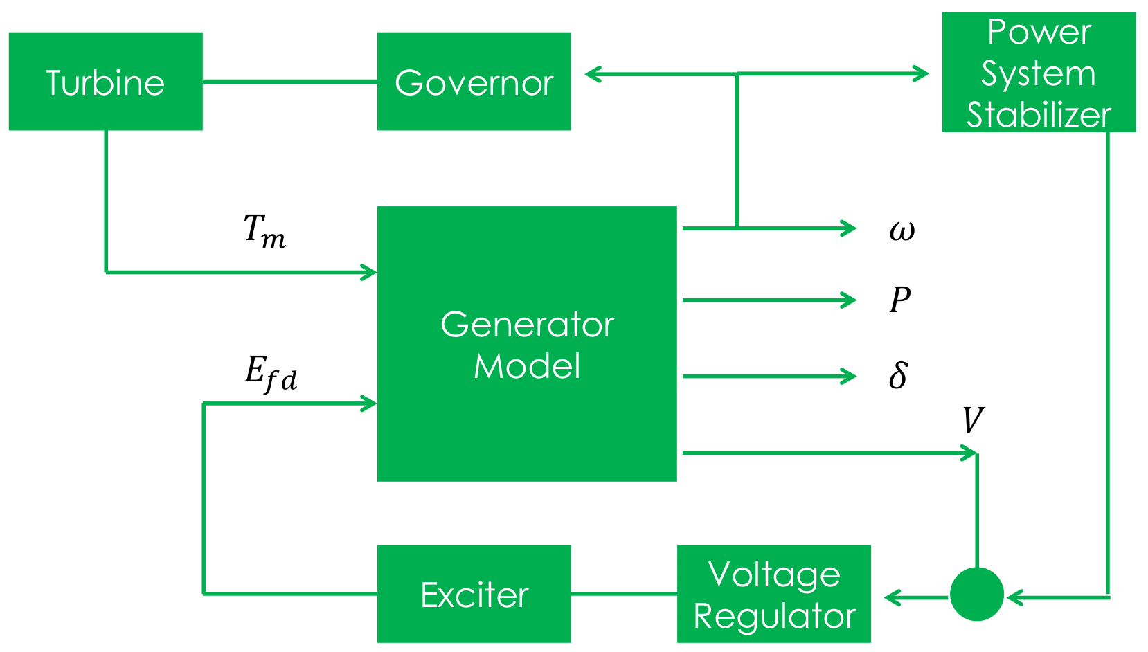
Fig. 1 Synchronous generator model with relevant controllers

Further details regarding the derivation of models can be found in [Pad08]. Notice that the power system stabilizer is not included in this version.

Algebraic Equations

By neglecting stator transients, the stator quantities contain only fundamental frequnecy component and the stator voltage equations appear as algebraic equations. With this, the use of steady-state relationships for representing the interconnecting transmission network is allowed. The neglection of stator transients together with network transients is necessary for stability analysis of practical power systems consisting of thousands of buses and hundreds of generators.

Stator Algebraic Equation

\[\begin{split}\begin{aligned} E_q^{''} & = X_{ad}^{''} \Big(\frac{\psi_{f}}{X_{fl}} + \frac{\psi_{h}}{X_{hl}}\Big) \\ E_d^{''} & = -X_{aq}^{''} \Big(\frac{\psi_{g}}{X_{gl}} + \frac{\psi_{k}}{X_{kl}}\Big) \\ X_q^{''} & = X_{aq}^{''} + X_l \\ X_d^{''} & = X_{ad}^{''} + X_l \\ v_q + jv_d & = (V_q + jV_d)e^{-j\delta} \\ \begin{bmatrix} i_q \\ i_d \\ \end{bmatrix} & = \frac{1}{R_a^2 + X_{d}^{''}X_{q}^{''}} \begin{bmatrix} R_a & X_{d}^{''} \\ -X_{q}^{''} & R_a \\ \end{bmatrix} \begin{bmatrix} E_q^{''} - v_q \\ E_d^{''} - v_d \\ \end{bmatrix} \\ T_e & = E_q^{''}i_q + E_d^{''}i_d + (X_{ad}^{''} - X_{aq}^{''})i_di_q \\ \psi_{ad} & = X_{ad}^{''}i_d + E_q^{''} \\ \psi_{aq} & = X_{aq}^{''}i_q - E_d^{''} \\ \psi_{at} & = (V_q + jV_d) + (R_a + jX_l)(i_q+ji_d) \\ \psi_{Id} & = A_{sd}e^{B_{sd}(\psi_{at}-\psi_{Td})} \\ \psi_{Iq} & = A_{sq}e^{B_{sq}(\psi_{at}-\psi_{Tq})} \\ K_{sd} & = \frac{\psi_{at}}{\psi_{at}+\psi_{Id}} \\ K_{sq} & = \frac{\psi_{at}}{\psi_{at}+\psi_{Iq}} \\ X_{ads} & = K_{sd}X_{ad} \\ X_{aqs} & = K_{sq}X_{aq} \\ F_{d} & = \frac{1}{\frac{1}{X_{ads}} + \frac{1}{X_{fl}} + \frac{1}{X_{hl}}} = X_{ad}^{''}\\ F_{q} & = \frac{1}{\frac{1}{X_{aqs}} + \frac{1}{X_{gl}} + \frac{1}{X_{kl}}} = X_{aq}^{''} \end{aligned}\end{split}\]

where $E_q^{''}, E_d^{''}$ are the q-axis and d-axis subtransient voltage; $X_q^{''}, X_d^{''}$ are the saturated q-axis and d-axis subtransient reactance; $T_e$ is the electrical torque; $\psi_{ad}, \psi_{aq}$ are the d-axis and q-axis component of mutual flux linkage; $\psi_{at}$ is the saturated value of resultant air-gap flux linkages; $K_{sq}$, $K_{sd}$ are the q-axis and d-axis saturation factor; $X_{ad}, X_{aq}$ are the unsaturated d-axis and q-axis mutual synchronous reactance; $X_{ads}, X_{aqs}$ are the saturated value of $X_{ad}, X_{aq}$.

Network Algebraic Equation

Since the time constants of these elements are relatively small compared to the mechanical time constants, the network transients are neglected and the network is assumed to be in sinusoidal steady state. Using the $Y_{bus}$ matrix, the bus voltage can be obtained with the current injections from load and generation buses.

\[\begin{split}\begin{aligned} I_{bus} & = I_{Lr} + \mathbf{j}I_{Li} \quad \text{for load buses} \\ I_{bus} & = I_q + jI_d = \frac{E_q^{''} + j(E_q^{''} + E^{\text{dummy}})}{R_a + jX^{''}_{d}}e^{j\delta} \quad \text{for generator buses} \\ V_{bus} & = Y_{bus}^{-1}I_{bus}\end{aligned}\end{split}\]

Load Algebraic Equation

\[\begin{split}\begin{aligned} Y_L & = \frac{P_{L0} - jQ_{L0}}{V_0^2} \\ P_L & = a_1P_{L0} + a_2 \Big( \frac{P_{L0}}{V_0} \Big)V + a_3 \Big( \frac{P_{L0}}{V_0^2} \Big)V^2 \\ Q_L & = b_1Q_{L0} + b_2 \Big( \frac{Q_{L0}}{V_0} \Big)V + b_3 \Big( \frac{Q_{L0}}{V_0^2} \Big)V^2 \\ S_L & = P_L + j Q_L \\ I_L & = VY_L - \Big(\frac{S_L}{V}\Big)^* \\ F_r & = real(I_L) \\ F_i & = imag(I_L) \end{aligned}\end{split}\]

where $V_0$ is the nominal load bus voltage magnitude; $I_L$ in general represents load currents, which is related to load power; $P_{L0}, Q_{L0}$ are nominal values of active and reactive components of load powers at nomial voltage $V_{0}$; The coefficients $a_1$, $a_2$ and $a_3$ are the fractions of the constant power, constant current and constant impedance components in the active load powers, respectively. Similarly, the coefficients $b_1$, $b_2$ and $b_3$ are defined for reactive load powers.

It should be noted that $a_1 + a_2 + a_3 = 1$ and $b_1 + b_2 + b_3 = 1$. Also notice that the active and reactive components of load powers are represented separately as static voltage dependent models. As illustrated before, the values of $F_r$ and $F_i$ are substituted in the load dynamic equation to avoid the iterative solution. Similarly, further details regarding the derivation can be found in [Pad08]. The example of the IEEE New England test network is shown in Fig. 2.

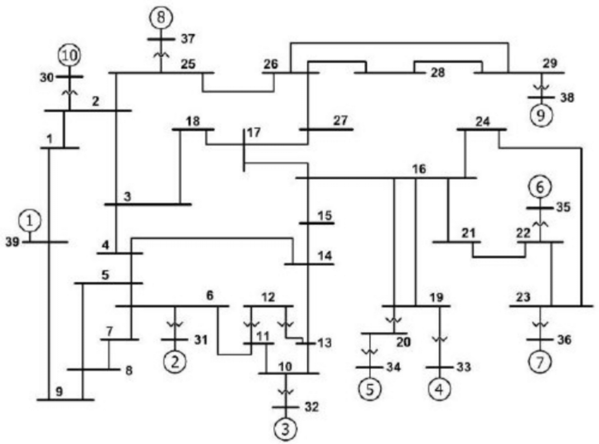
Fig. 2 Example of the New England test network: 39-bus and 10-generator

Dynamic Simulation

This section describes the procedures and solution approach for performing power system dynamic simulations.

Initial Condition Calculations

To start the dynamic simulations, the calculation of initial conditions requires the solution of the power flow problem which obtains a set of feasible steady-state system conditions. From the power flow analysis, the power output of generator and bus voltage phasor can be obtained.

Synchronous Generator Initial Conditions

The calculation of unsaturated parameters: First, we derive the value of other parameters with given parameters (e.g., subtransient and transient inductance). The derived parameters include $[X_{ad},X_{aq},X_{fl},X_{hl},R_f,R_h,X_{gl},X_{kl},\\R_g,R_k]$.
The calculation of saturation: From the power flow solution, one obtains the bus voltage ($V_{g,0}$), current ($I_{g,0}$) and power ($P_{g,0}/Q_{g,0}$) at the generator buses. With this, obtain the air-gap voltage as $E^{\text{air}} = V_{g,0} + jX_lI_{g,0}$. Then, using saturation parameters (satData), calculate the saturation coefficient $K_{sd},K_{sq}$. Finally, update the derived parameters to appropriately reflect the saturation effect as follows:

\[\begin{split}\begin{aligned} X_{ad} & = K_{sd}X_{ads} \\ X_{aq} & = K_{sq}X_{aqs} \\ X_{d} & = X_{ad} + X_l \\ X_{q} & = X_{aq} + X_l \\ X_{ad}^{''} & = \frac{1}{\frac{1}{X_{ad}} + \frac{1}{X_{fl}} + \frac{1}{X_{hl}}} \\ X_{aq}^{''} & = \frac{1}{\frac{1}{X_{aq}} + \frac{1}{X_{gl}} + \frac{1}{X_{kl}}} \\ X_{ds}^{''} & = X_{ad}^{''} + X_l \\ X_{qs}^{''} & = X_{aq}^{''} + X_l \end{aligned}\end{split}\]
The calculation of initial values for state variables:

Compute:

\[\begin{split}\begin{aligned} E_q & = V_{g,0} + \textbf{j}X_qI_{g,0} \\ \delta_0 & = \angle E_q \\ i_q + \textbf{j}i_d & = I_{g,0}e^{-\textbf{j}\delta_0} \\ v_q + \textbf{j}v_d & = V_{g,0}e^{-\textbf{j}\delta_0} \\ \psi_d & = v_q \\ \psi_d & = -v_d \end{aligned}\end{split}\]

\[\begin{split}\begin{aligned} i_{f,0} & = \frac{\psi_d - X_di_d}{X_{ad}} \\ E_{fd,0} & = X_{ads}i_{f,0} \end{aligned}\end{split}\]

\[\begin{split}\begin{aligned} \psi_{ad} & = \psi_{d} - X_li_d \\ \psi_{aq} & = \psi_{q} - X_li_q \end{aligned}\end{split}\]

\[\begin{split}\begin{aligned} \psi_{f,0} & = \psi_{ad} + \frac{X_{fl}}{X_{ads}}E_{fd,0} \\ \psi_{h,0} & = \psi_{ad} \\ \psi_{g,0} & = \psi_{aq} \\ \psi_{k,0} & = \psi_{aq} \end{aligned}\end{split}\]

\[\begin{aligned} T_{m,0} & = P_{g,0} \end{aligned}\]

\[\begin{split}\begin{aligned} E_q^{''} & = X_{ad}^{''} \Big( \frac{\psi_f}{X_{fl}} + \frac{\psi_h}{X_{hl}} \Big) \\ E_d^{''} & = -X_{ad}^{''} \Big( \frac{\psi_g}{X_{gl}} + \frac{\psi_k}{X_{kl}} \Big) \\ T_{m0} & = E_q^{''}i_q + E_d^{''}i_d + i_di_q(X_{ad}^{''} - X_{aq}^{''}) \end{aligned}\end{split}\]

\[\begin{aligned} E^{\text{dum}}_0 & = -(X_{q}^{''} - X_{d}^{''})i_q \end{aligned}\]

\[\begin{aligned} Y_{bus}(gen,gen) & = Y_{bus}(gen,gen) + \frac{1}{R_a(gen) + \textbf{j}X_d^{''}(gen)} \end{aligned}\]

\[\begin{aligned} Y_{bus}(load,load) & = Y_{bus}(load,load) + \frac{P_{L0}(load) - \textbf{j}Q_{L0}(load)}{|V(load)|^2} \end{aligned}\]

Then, setting $\omega_0=0, X_{ad0}^{''}=X_{ad}^{''}, X_{aq0}^{''}=X_{aq}^{''}$, we obtain $X_0=[\delta_0,\omega_0,\psi_{f0},\psi_{h0},\psi_{g0},\\ \psi_{k0},E^{\text{dum}}_0,X_{ad0}^{''},X_{aq0}^{''}]$. Also, one can obtain $E_{fd0},T_{m0}$.

Excitation System Initial Conditions

The calculation of initial values for state variables: With $V_{g0}$, $E_{fd0}$ from generator initial conditions and exciter parameters, compute:

\[\begin{split}\begin{aligned} V_{2,0} & = \frac{K_F}{T_F}E_{fd,0} \\ V_{1,0} & = |V_{g,0}| \\ V_{RR} & = (K_E + A_Ee^{B_EE_{fd,0}})E_{fd,0} \\ V_{R,0} & = K_A \big( \frac{V_{RR}}{K_A} - \frac{K_F}{T_F}E_{fd,0} - V_{2,0} \big) \end{aligned}\end{split}\]

Governor Initial Conditions

The $T_{m,0}$ becomes the governor set point (i.e. $T_{m,0} = P_c = P_{sv,0}$) and is the input for the initial condition of turbine.

Turbine Initial Conditions

Here, simply $T_{m,0}=P_{sv,0}$.

Solution Approach

There are basically two approaches used in power system simulation packages. One approach, called partitioned-explicit (PE) solution, solves the differential and the algebraic equations separately in an alternating manner. The second approach solves the differential equations along with the algebraic equations simultaneously.

Partitioned-explicit (PE) method
Simultaneous-implicit (SI) method

The PE approach with explicit integration is the traditional approach used widely in production-grade stability programs. Therefore, we only focus on the partitioned solution approach with an explicit integration method. Initially, at $t=0$, the values of the state variable and the algebraic variables are known, and the system is in steady state and the time derivatives $\pmb{f}$ are zero.

Following a disturbance, the state variable $\pmb{x}$ cannot change instantly, whereas the algebraic variables can change instantaneously. Therefore, the algebraic equations are solved solved first to give $\pmb{V}_{bus}$ and $\pmb{I}_{bus}$, and other non-state variables of interest at $t=0^{+}$. Then, the $\pmb{f}$ is computed by using the known values of $\pmb{x}$ and $\pmb{V}_{bus}$. We illustrate this process based on the fourth order Runge-Kutta (RK-4) method.

Step 1: Incorporate the system disturbance and solve for $V(0^{+}),I(0^{+})$.
Step 2: Using the value of $V(0^{+}),I(0^{+})$, integrate the differential equations to obtain $k_1$.
Step 3: Then, algebraic equaiotns are solved with $k_1$ and $V(0^{+}),I(0^{+})$ to compute $V(0^{+})^1,I(0^{+})^1$.
Step 4: Using the value of $V(0^{+})^1,I(0^{+})^1$, integrate the differential equations to obtain $k_2$, and this is applied successively until $k_4$ and $V(0^{+})^4,I(0^{+})^4$.
Step 5: Update the solution $x_{1} = x_{0} + \frac{1}{6}(k_1 + 2k_2 + 2k_3 + k_4)$.
Step 6: Go to Step 1 and solve for $V(1),I(1)$ from the algebraic equations.

The advantages of the partitioned approach with explicit integration are programming flexibility, and simplicity, reliability, and robustness. Its disadvantage is numerical instability.

Parareal Algorithm

To implement the aforementioned partitioned-explicit solution process, which is widely applied in power system commercial simulation softwares, $RAPID$ employs the Parareal algorithm [G+16] that belongs to the class of temporal decomposition methods and can highly utilize high-performance parallel computing platforms. It has become popular in recent years for long time transient simulations and demonstrated its potential to reduce the wall-clock time of the simulations significantly, which is crucial for “faster than real-time simulations.” In a simplified way, the Parareal algorithm decomposes the whole simulation period into smaller time intervals such that the evolution of each independent sub-interval is carried out in parallel and completed after a number of iterations between a coarse approximate solution and a fine true solution over the entire period. Its computational performance is heavily dependent on the number of iterations, and for fast convergence, it is crucial to select the coarse operator that is reasonably accurate and fast.

To solve these sub-intervals independently, initial states for all sub-intervals are required, which are provided by a less accurate but computationally cheap numerical integration method (coarse operator). The more accurate but computationally expensive numerical integration method (fine operator) is then used to correct the evolution of each independent sub-interval in parallel. As an example, consider an initial value problem of the form:

\[\begin{split}\begin{aligned} \label{eq:IVP} \dot{x} & = f(x,t) \\ x(t_0) & = x_0 \quad \text{with} \,\,\, t_0 \leq t \leq T\end{aligned}\end{split}\]

Then, it divides the time interval $[t_0,T]$ into $N$ sub-intervals $[t_j,t_{j+1}]$ such that $[t_0,T]=[t_0,t_1]\cup[t_1,t_2]\cup\ldots\cup[t_{N-1},t_{N}]$. For simplicity, assume that the size of $t_{n+1}-t_{n} = \Delta T_n$ is equivalent to each other for all $0 \leq n < N$ (i.e., $\Delta T = \Delta T_n$).

Parareal Implementation

The following steps roughly describe the standard Parareal implementation. Denote $x^{\text{fine}}$ and $x^{\text{coarse}}$ as the system states obtained from fine operator and coarse operator, respectively. $x^*$ is used to denote the corrected coarse solution.

Define two numerical operators, Fine and Coarse, using time steps $\delta t$ and $\Delta t$, respectively from initial state $x_{n-1}$ at time $t_{n-1}$.

\[\begin{split}\begin{aligned} Fine: x^{\text{fine}}_{n} = F_{\delta t}(t_{n-1},x_{n-1}) \\ Coarse: x^{\text{coarse}}_{n} = C_{\Delta t}(t_{n-1},x_{n-1}) \end{aligned}\end{split}\]
Generate an initial coarse solution using the coarse operator in serial

\[\begin{split}\begin{aligned} x_{n}^{*,0} = x^{\text{coarse},0}_{n} = C_{\Delta t}(x_{n-1}^{*,0}) & \quad n = [1,,,.,N] \\ & \text{Set} \quad x^{*,1}_{0} = x^{*,0}_{0} \end{aligned}\end{split}\]

where the superscript denotes the iteration count and $x^{*,0}_{0}$ is the given initial point at $T=0$.
Iteration starts $k=1$. Propagate fine solution in parallel over each time sub-intervals $[T_{n-1},T_n)$ using the find operator

\[\begin{aligned} x^{\text{fine},k}_{n} = F_{\delta t}(x_{n-1}^{*,k-1}) \quad n = [1,,,.,N] \end{aligned}\]

where $x^{\text{fine},k}_{n}$ denotes the solution at $t_n$.
Update the coarse solution in serial

for $n = k:N$

\[ \begin{align}\begin{aligned}\begin{split} \begin{aligned} \label{eq:update_coarse} x^{\text{coarse},k}_{n} & = C_{\Delta t}(x_{n-1}^{*,k}) \\ x^{*,k}_{n} & = x^{\text{coarse},k}_{n} + x^{\text{fine},k}_{n} - x^{\text{coarse},k-1}_{n} \end{aligned}\end{split}\\end\end{aligned}\end{align} \]
Go to Step 3 and update the coarse solution iteratively until $x^{*,k}_{n} - x^{*,k-1}_{n} \leq tol$ for $n = [1,,,.,N]$.

Understanding of Parareal Algorithm

To understand the behavior of this algorithm, consider the updated coarse solution at n = 1 after the first iteration (k = 1); that is, $x^{*,1}_1 = x_1^{\text{coarse,1}} + x_1^{\text{fine,1}} - x_1^{\text{coarse,0}}$. Notice that the updates coarse solution at t1 is corrected to the fine solution as $x^{*,1}_1 = x_1^{\text{fine,1}}$ since $x^{\text{coarse},1}_1 = x_1^{\text{coarse,0}}$. Therefore, all the coarse values should be corrected to fine values (true solution) in $N$ iterations. This is same as the fine operator is applied sequentially for all $N$ intervals. Thus, the speedup can be obtained only if the Parareal iteration $k$ is less than $N$. That is, $k < N$. This means that the ideal speed up of Parareal is $\frac{N}{k}$ assuming inexpensive coarse solver and other factors related to the parallelization are negligible. In addition, note that Step 4 updates the coarse solution at $t_n$ from $k$ to $N$ since the updated coarse solutions $x_1^{*},x_2^{*},...,x_{k-1}^{*}$ have been corrected to the true solutions in $k$ iterations.

One can consider many different ways to construct the coarse operator, and common approaches are: 1) the use of a larger time step than the fine operator, 2) the use of a different, but faster solver than that of the fine operator, and 3) the use of a simpler or reduced system model based on the properties of the underlying physics governing the behavior of the system. The graphical structure of the Parareal algorithm is illustrated in Fig. 3.

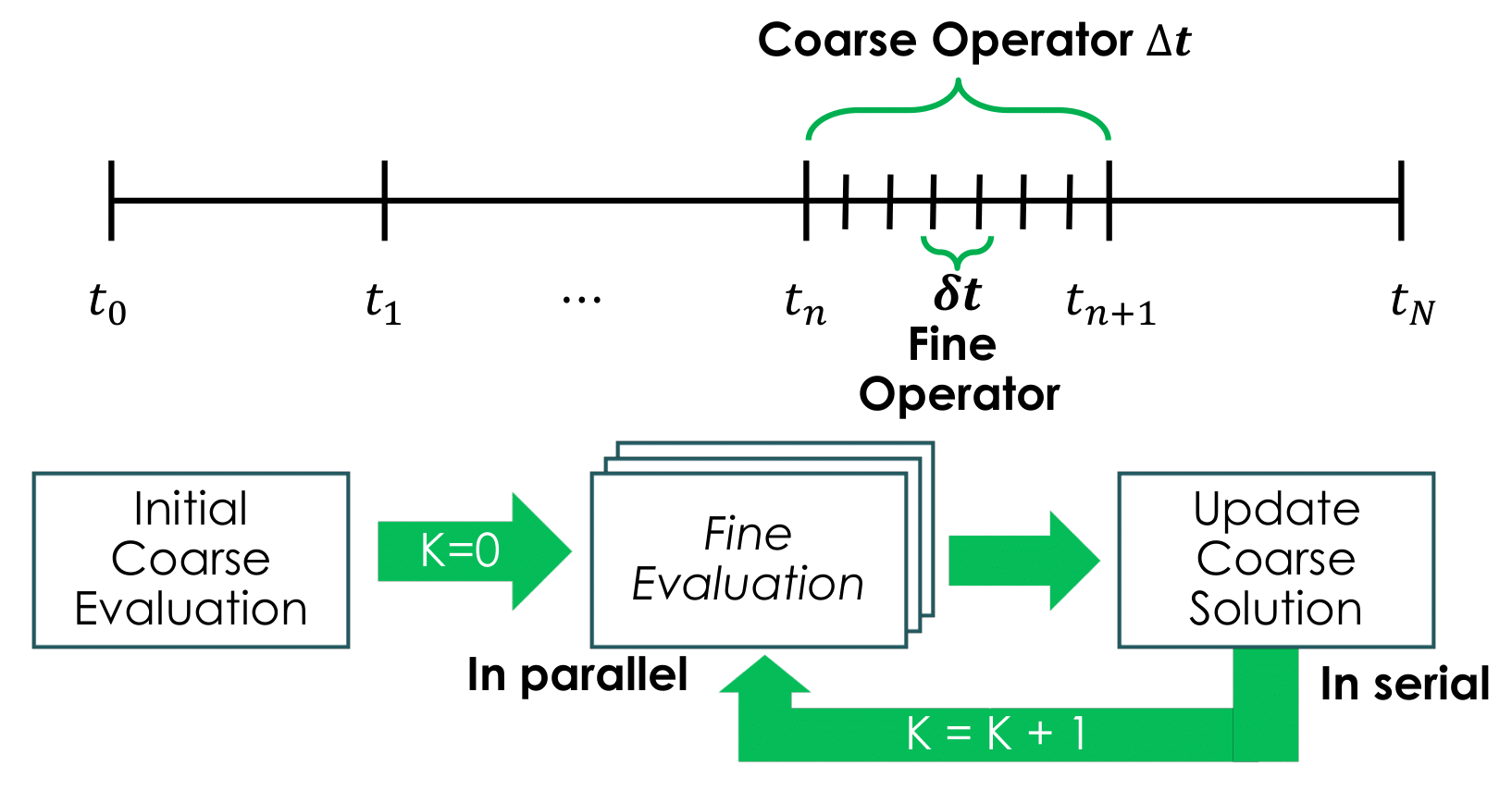
Fig. 3 Parareal algorithm

For the Parareal algorithm, this toolbox employs the distributed Parareal algorithm [Aub11] that considers the efficient scheduling of tasks, which is an improved version of the usual Parareal algorithm from a practical perspective. In the distributed algorithm, the coarse propagation is also distributed across all processors, which enables overlap between the sequential and parallel portions and mitigates the memory requirement for processors.

To evaluate the computational efficiency of Parareal algorithm, one might consider the ideal speedup of Parareal algorithm assuming ideal parallelization and negligible communication time. In the distributed Parareal algorithm, the ideal runtime $(t^{\text{ideal}})$ of Parareal algorithm can be given as:

\[\begin{aligned} t^{\text{ideal}} = T_c + \frac{k}{N}(T_f + T_c) \end{aligned}\]

where $N$ and $k$ represent the number of processors used in the fine operator and the number of Parareal iterations required for convergence, respectively; $T_c$ and $T_f$ refer to the coarse and fine propagation times, respectively over the whole simulation time period.

$\textsf{para\_real.py}$

The main python code to runt RAPID is para_real.py. An example
command line to run the simulation is following:
mpiexec -n 50 python para_real.py 0.0 0.2 –nCoarse 10 –nFine 100 –tol 0.01 –tolcheck maxabs –debug 1 -o result.csv
Necessary arguments are

50: the number of processors for parallel computing of the fine operator.
0: start time.
0.2: end time.

Optional arguments are

–nCoarse: the number of time intervals for the coarse operator.
–nFine: the number of time intervals for the fine operator.
–tol: tolerance for convergence. The default is 1.0.
–tolcheck: method for convergence check. The default is L2.
–debug: debug printout.
-o: write results to result.csv.

In the result.csv file, results are formatted in the csv form. The first column corresponds to the simulation time and other columns correspond to the solution values of state and algebraic variables. Each row corresponds to each time step.

\[\begin{split}\begin{aligned} \begin{bmatrix} Col1 & Col2 & \cdots & ColM \\ \hline t_0 & Sol_1(t_0) & \cdots & Sol_{M-1}(t_0) \\ t_1 & Sol_1(t_1) & \cdots & Sol_{M-1}(t_1) \\ \cdots & \cdots & \cdots & \cdots \\ t_N & Sol_1(t_N) & \cdots & Sol_{M-1}(t_N) \\ \end{bmatrix}\end{aligned}\end{split}\]

Solution Method

This section describes a variety of solution methods which is employed in the coarse operator and fine operator of the Parareal algorithm. One approach is based on the standard numerical predictor-corrector method, and another approach is based on the semi-analytical solution method.

Standard Numerical Iteration Method

Midpoint-Trapezoidal Predictor-Corrector

Based on the results in [G+16], the following Midpoint-Trapezoidal predictor-corrector (Trap) method is selected as the standard numerical predictor-corrector method to be used as the coarse operator of Parareal algorithm. This Trap method serves as the standard coarse operator and is compared with two SAS methods that will be discussed in the subsequent sections.

Coarse Operator:

\[\begin{split}\begin{aligned} % \label{eq:corase} \nonumber Midpoint & \,\, Predictor: \\ x^{j}_{n+1} & = x^{j}_{n} + \Delta t f\Big(t_n+\frac{\Delta t}{2},x_n + \frac{1}{2}f(t_n,x_n) \Big) \\ Trapezoidal & \,\, Corrector: \\ x^{j+1}_{n+1} & = x^{j}_{n} + \frac{\Delta t}{2}\Big[f(t_n,x_n) + f(t_{n+1},x^{j}_{n+1}) \Big] \end{aligned}\end{split}\]

For the Trap method, only one iteration $(j=1)$ is used to obtain an approximate solution in the simulations.

the Runge-Kutta 4th Order Method

For the fine operator, the Runge-Kutta 4th order (RK-4), widely used in power system dynamic simulations, is employed. This RK-4 method has remained unchanged as the fine operator of Parareal algorithm for the dummy coil model.

Fine Operator:

\[\begin{split}\begin{aligned} k_1 & = f(t_n,x_n), \,\, k_2 = f\Big( t_n+\frac{\delta t}{2},x_n+\frac{\delta t}{2}k_1 \Big) \\ k_3 & = f\Big( t_n+\frac{\delta t}{2},x_n+\frac{\delta t}{2}k_2 \Big) \\ k_4 & = f\Big( t_n+\delta t,x_n+\delta tk_3 \Big) \\ x_{n+1} & = x_n + \frac{1}{6}[k_1 + 2k_2 + 2k_3 + k_4] \end{aligned}\end{split}\]

Network equations are solved within each time step for the both coarse and fine operators in order to mitigate interface errors due to alternating solution.

Semi-Analytical Solution Method

Besides the standard numerical iteration methods, semi-analytical solution (SAS) has been proposed in recent years for fast power system simulations. Generally, the SAS refers to power series or closed-form solutions for approximating solutions of nonlinear differential equations. SAS in a form of an explicit expression can be derived offline once for given system conditions, and then evaluated in the online stage without iterations. SAS methods have been widely applied to solve nonlinear ordinary differential equations (ODEs) and DAE problems in the applied sciences and engineering [23]. The SAS-based approach is a powerful analytical technique for strongly nonlinear problems. It can provide a RAPID convergence to a solution, and thus has shown the potential for fast power system simulations.

This toolbox utilizes two promising time-power series-based SAS methods; Adomian decomposition method (ADM) [G+17], [DRBW12] and Homotopy Analysis method (HAM) [Lia03], [DG19]. In the time-power series-based SAS methods, the true solution $x(t)$ to the initial value problem of [eq:IVP] can be analytically represented as an infinite series []:

\[\begin{aligned} \label{eq:SAS1} x(t) = \sum_{i=0}^{\infty} a_i (t-t_0)^i = a_0 + a_1(t-t_0) + \cdots\end{aligned}\]

where $t_0$ represents the initial time; $a_0$ indicates the initial state $x_0$; and $a_i$ for $i \geq 1$ depends on $a_0$ and system parameters. The SAS method approximates the solution $x(t)$ by truncating higher order terms of the true solution [eq:SAS1] as follows:

\[\begin{aligned} \label{eq:SAS2} x(t) \approx x_{SAS}^{m}(t) = \sum_{i=0}^{m} a_i (t-t_0)^i \end{aligned}\]

where $m$ is the order of the SAS $x_{SAS}^{m}(t)$.

Notice that the basic idea of SAS methods is to shift the computational burden of deriving an approximate but analytical solution, which preserves accuracy for a certain time interval, to the offline stage that mathematically derives unknown coefficients $a_1, a_2,...,a_m$. Then, in the online stage, values are simply plugged into symbolic SAS terms, which are already derived offline, over consecutive time intervals until the end of the whole simulation period. This allows for a very fast online simulation task since no numerical iteration is needed. There can be multiple ways to derive such unknown coefficients $a_1, a_2,...,a_m$. The following subsections discuss two SAS methods to obtain these terms for DEs of power systems.

Adomian Decomposition Method

This section briefly reviews the basic concept of ADM. Consider a nonlinear ordinary differential equation (ODE) in the following form:

\[\begin{aligned} \label{eq:ADM0} Lx = -Rx - N(x) + g\end{aligned}\]

where $L = \frac{d}{dt}$ and $L^{-1} = \int_{0}^{t}dt$; $x$ is the state variable of the system; $R$ and $N$ are the linear and nonlinear operator, respectively; and $g$ is the constant term. One should identify the highest differential operator, constant terms, linear and nonlinear function in the ODE. With this, one might get the following to solve for $x$:

\[\begin{aligned} \label{eq:ADM1} x = x_0 + L^{-1}g - L^{-1}Rx - L^{-1}N(x) \end{aligned}\]

where the inverse operator can be regarded as $L^{-1}=\int_{0}^{t}dt$ and $x_0$ is the given initial condition. Now, assume that the solution $x(t)$ can be presented as an infinite series of the form:

\[\begin{aligned} x(t) = \sum_{n=0}^{\infty} x_{n}(t) \end{aligned}\]

and then decompose the nonlinear operator $N(x)$ into infinite series:

\[\begin{aligned} \label{eq:ADM2} N(x) = \sum_{n=0}^{\infty} A_{n}\end{aligned}\]

where $A_{n}$ are called the Adomain polynomials. Suppose the nonlinear function $N(x) = f(x)$. Adomian polynomials are obtained using the following formula:

\[\begin{aligned} A_{n}(x_0,x_1,x_2,...,x_n) = \frac{1}{n!}\Big[\frac{d^n}{d\lambda^n}\sum_{\infty}^{i=0} \lambda^i x_i \Big] \Big|_{\lambda=0}\end{aligned}\]

where $\lambda$ is a grouping parameter. Then, we substitute the Adomian series, [eq:ADM1] and [eq:ADM2], in [eq:ADM0], which gives the solution for $x(t)$ as:

\[\begin{aligned} x(t) = \sum_{n=0}^{\infty} x_{n} = x_0 + L^{-1}g - L^{-1}R\sum_{n=0}^{\infty} x_{n} - L^{-1}\sum_{n=0}^{\infty} A_{n}\end{aligned}\]

From this, we can obtain the terms of the ADM in power series forms as follows:

[eq:ADM3]

\[\begin{split}\begin{aligned} x_{0}(t) & = x(0) \\ x_{1}(t) & = L^{-1}g -L^{-1}Rx_{0} - L^{-1}A_{0} \\ x_{2}(t) & = -L^{-1}Rx_{1} - L^{-1}A_{1} \\ & \quad \quad \quad \colon \\ x_{n+1}(t) & = -L^{-1}Rx_{n} - L^{-1}A_{n}\end{aligned}\end{split}\]

The AMD method provides a fast convergence series, and thus the approximate solution by the truncated series $\sum_{n=0}^{m}x_n = x_{SAS}^{m}(t)$ can serve as a good practical solution. Here, the coefficients $a_0,a_1,...,a_m$ in [eq:SAS2] correspond to the terms $x_0,x_1,...,x_m$ in [eq:ADM3].

In particular, we employ multi-stage approach, applying ADM over multiple intervals of time, to improve the convergence region of power series ODE solution using ADM; this is referred to as the multistage ADM (MADM). The MADM uses the ADM to approximate the dynamical response in a sequence of time intervals $[0,t_1],[t_1,t_2],...,[t_{N-1},t_{N}]$. Note that the solution at tn becomes an initial condition in the interval $[t_{n},t_{n+1}]$. This toolbox uses the MADM as one of the coarse operators to obtain an approximation solution $x(t)$ with the equal time step $\Delta t$ for all intervals, which is the step size of integration for the coarse operator.

In addition, the derivation of first few polynomials is given as follows:

[eq:ADM4]

\[\begin{split}\begin{aligned} A_{0} & = f(x_0) \\ A_{1} & = \frac{1}{1!} \frac{d}{d\lambda} \Big[f(x_0 + x_1\lambda^1 + x_2\lambda^2 + \cdots ) \Big]\Big|_{\lambda=0} \\ & = 1 f^{'}(x_0 + u^1\lambda^1 + \cdots ) (x_1 + 2 x_2 \lambda + \cdots ) \quad \text{by chain rule} \\ & = f^{'}(x_0)x_1 \\ A_{2} & = \frac{1}{2!} \frac{d^2}{d\lambda^2} \Big[f(x_0 + x_1\lambda^1 + x_2\lambda^2 + \cdots ) \Big]\Big|_{\lambda=0} \\ & = \frac{1}{2!} \frac{d}{d\lambda} \Big[f^{'}(x_0 + u^1\lambda^1 + \cdots ) (x_1 + 2 x_2 \lambda + \cdots ) \Big]\Big|_{\lambda=0} \\ \nonumber & = \frac{1}{2!} \Big[f^{''}(x_0 + u^1\lambda^1 + \cdots ) (x_1 + 2 x_2 \lambda + \cdots ) (x_1 + 2 x_2 \lambda + \cdots ) \\ & \quad \quad \,\, + f^{'}(x_0 + u^1\lambda^1 + \cdots ) (2 x_2 + \cdots ) \Big]\Big|_{\lambda=0} \quad \text{by product rule} \\ & = \frac{1}{2!} \Big[ f^{''}(x_0)x_1^2 + 2f^{'}(x_0)x_2 \Big] \\ A_{3} & = \frac{1}{3!} \Big[ f^{'''}(x_0)x_1^3 + 3!f^{''}(x_0)x_1x_2 + 3!f^{'}(x_0)x _3 \Big] \quad \text{by similar step}\end{aligned}\end{split}\]

The derivation of MADM terms for each device:

The following descriptions detail the derivation of MADM terms for each device. The following steps summarize the development of the MDAM:

Recognize linear, nonlinear, and constant terms of differential equations according to [eq:ADM1].
Find nonlinear terms, and approximate them using Adomian polynomial [eq:ADM4]. If there is no nonlinear term, this step is not needed.
Obtain the MADM terms $(x_{0},x_1,...,x_m)$ based on [eq:ADM3] and integrate each term analytically.
Obtain the closed form approximate solution for the desired number of terms $m$.

\[\begin{aligned} x(\Delta t) & = x_{0} + x_{1}\Delta t + ... + x_{m} \Delta t^m \end{aligned}\]

We apply these steps to each device. As an example, we describe the derivation of a few terms as follows:

Turbine:

\[\begin{split}\begin{aligned} \dot{T_{m}} & = \frac{1}{T_{ch}} (-T_{m} + P_{sv} ) \\ T_{m}(t) & = T_{m}(0) + \frac{1}{T_{ch}} \int_{0}^{\Delta t}(-T_m + P_{sv}) dt \\ T_{m,0} & = \pmb{T_{m}(0)} \\ T_{m,1} & = \frac{1}{T_{ch}} \int_{0}^{\Delta t} (-T_{m}(0) + P_{sv}(0))dt = \pmb{\frac{1}{T_{ch}}(-T_{m}(0) + P_{sv}(0)) } \Delta t \\ T_{m,2} & = \frac{1}{T_{ch}} \int_{0}^{\Delta t} (-T_{m,1} + P_{sv,1})dt \\ \nonumber & = \frac{1}{T_{ch}} \int_{0}^{\Delta t} \Big( - \frac{1}{T_{ch}} (-T_{m}(0) + P_{sv}(0))\Delta t \\ & \quad\quad\quad\quad\quad\quad + \frac{1}{T_{sv}} (-P_{sv}(0) + P_c - \frac{1}{R_d}\omega(0)) \Delta t \Big) dt \\ & = \frac{1}{T_{ch}} \Big[ -\frac{1}{2}T_{m,1}t^2 + \frac{1}{2}P_{sv,1}t^2 \Big]^{\Delta t}_{0} \\ & = \pmb{\frac{1}{T_{ch}} \Big( -\frac{1}{2}T_{m,1} + \frac{1}{2}P_{sv,1} \Big)} \Delta t^2 \\ T_{m,3} & = \frac{1}{T_{ch}} \int_{0}^{\Delta t} (-T_{m,2} + P_{sv,2})dt \\ T_{m,4} & = \cdots \end{aligned}\end{split}\]
Governor:

\[\begin{split}\begin{aligned} \dot{P_{sv}} & = \frac{1}{T_{sv}} (-P_{sv} + P_c - \frac{1}{R_d}\omega ) \\ P_{sv}(t) & = P_{sv}(0) + \frac{1}{T_{sv}} \int_{0}^{\Delta t}(-P_{sv} + P_c - \frac{1}{R_d}\omega) dt \\ P_{sv,0} & = \pmb{P_{sv}(0)} \\ P_{sv,1} & = \frac{1}{T_{sv}} \int_{0}^{\Delta t} (-P_{sv}(0) + P_c - \frac{1}{R_d}\omega(0) )dt \\ & = \pmb{\frac{1}{T_{sv}}(-P_{sv}(0) + P_c - \frac{1}{R_d}\omega(0))} \Delta t \\ P_{sv,2} & = \frac{1}{T_{sv}} \int_{0}^{\Delta t} (-P_{sv,1} - \frac{1}{R_d}\omega_{1})dt \\ & = \frac{1}{T_{sv}} \int_{0}^{\Delta t} (-P_{sv,1}\Delta t - \frac{1}{R_d}\omega_{1} \Delta t)dt \\ & = \pmb{\frac{1}{T_{sv}} \Big(-\frac{1}{2}P_{sv,1} - \frac{1}{2} \frac{1}{R_d}\omega_{1} \Big)} \Delta t^2 \end{aligned}\end{split}\]
Excitation:
1. The variable $E_{fd}$:
  
  \[\begin{split}\begin{aligned} \dot{E_{fd}} & = \frac{1}{T_{E}} (-[K_E + A_E(e^{B_EE_{fd}})]E_{fd} + V_R) \\ E_{fd}(t) & = E_{fd}(0) + \frac{1}{T_{E}} \int_{0}^{\Delta t}(-K_EE_{fd} - A_E(e^{B_EE_{fd}})E_{fd} + V_R) dt \\ E_{fd}(t) & = E_{fd}(0) + \frac{1}{T_{E}} \int_{0}^{\Delta t}(-K_EE_{fd} - \sum_{n=0}^{\infty}A_{1,n} + V_R) dt \end{aligned}\end{split}\]
  
  Here, we define $A_1 = A_E(e^{B_EE_{fd}})E_{fd} = \sum_{n=0}^{\infty}A_{1,n}$. Therefore,
  
  \[\begin{split}\begin{aligned} E_{fd}(t) & = E_{fd}(0) + \frac{1}{T_{E}} \int_{0}^{\Delta t}(-K_EE_{fd} - \sum_{n=0}^{\infty}A_{1,n} + V_R) dt \\ E_{fd,0} & = \pmb{E_{fd}(0)} \\ E_{fd,1} & = \frac{1}{T_{E}} \int_{0}^{\Delta t}(-K_EE_{fd}(0) - A_{1,0} + V_R(0)) dt \\ E_{fd,1} & = \pmb{\frac{1}{T_{E}} (-K_EE_{fd}(0) - A_{1,0} + V_R(0)) } \Delta t \\ E_{fd,2} & = \frac{1}{T_{E}} \int_{0}^{\Delta t}(-K_EE_{fd,1} - A_{1,1} + V_{R,1})dt \\ & = \pmb{ \frac{1}{T_{E}} \Big( -\frac{1}{2}K_EE_{fd,1} - \frac{1}{2} (AA+BB)E_{fd,1} + \frac{1}{2} V_{R,1} \Big)} \Delta t^2 \end{aligned}\end{split}\]
  
  where $A_{1,0} = A_E(e^{B_EE_{fd}(0)})E_{fd}(0)$,
  
  and $A_{1,1} = \Big( A_E(e^{B_EE_{fd}(0)}) + B_EA_E(e^{B_EE_{fd}(0)})E_{fd}(0) \Big)E_{fd,1}$ = $(AA + BB)E_{fd,1}$, where $AA$ and $BB$ are newly introduced as parameters.
2. The variable $V_{2}$:
  
  \[\begin{split}\begin{aligned} \dot{V_{2}} & = \frac{1}{T_{F}} (-V_{2} + \frac{K_F}{T_F}E_{fd} ) \\ V_{2}(t) & = V_{2}(0) + \frac{1}{T_{F}} \int_{0}^{\Delta t} (-V_{2} + \frac{K_F}{T_F}E_{fd} )dt \\ V_{2,0} & = \pmb{V_{2}(0)} \\ V_{2,1} & = \pmb{ \frac{1}{T_{F}} (-V_{2}(0) + \frac{K_F}{T_F}E_{fd}(0)) \Delta t } \\ V_{2,2} & = \frac{1}{T_{F}} \int_{0}^{\Delta t} (-V_{2,1} + \frac{K_F}{T_F}E_{fd,1}) dt \\ & = \pmb{ \frac{1}{T_{F}} \Big(-\frac{1}{2}V_{2,1} + \frac{1}{2}\frac{K_F}{T_F}E_{fd,1} \Big)} \Delta t^2 \end{aligned}\end{split}\]
3. The variable $V_{1}$:
  
  \[\begin{split}\begin{aligned} \dot{V_{1}} & = \frac{1}{T_{R}} (-V_{1} + V_T ) \\ V_{1}(t) & = V_{1}(0) + \frac{1}{T_{R}} \int_{0}^{\Delta t} (-V_{1} + V_T )dt \\ V_{1,0} & = \pmb{V_{1}(0)} \\ V_{1,1} & = \pmb{\frac{1}{T_{R}} (-V_{1}(0) + V_T )} \Delta t \\ V_{1,2} & = \frac{1}{T_{R}} \int_{0}^{\Delta t} (-V_{1,1} ) dt \\ & = \pmb{\frac{1}{T_{R}} (-\frac{1}{2}V_{1,1} )} \Delta t^2 \end{aligned}\end{split}\]
4. The variable $V_{R}$:
  
  \[\begin{split}\begin{aligned} \dot{V_{R}} & = \frac{1}{T_{A}} \Big(-V_{R} + K_A\big(V^{\text{ref}}-V_1 - (\frac{K_F}{T_F}E_{fd}-V_2)\big) \Big) \\ \nonumber V_{R}(t) & = V_{R}(0) \\ & + \frac{1}{T_{A}} \int_{0}^{\Delta t} \Big(-V_{R} + K_A\big(V^{\text{ref}}-V_1 - (\frac{K_F}{T_F}E_{fd}-V_2)\big) \Big)dt \\ V_{R,0} & = \pmb{V_{R}(0)} \\ \nonumber V_{R,1} & = \frac{1}{T_{A}} \int_{0}^{\Delta t} \Big(-V_{R}(0) + K_AV^{\text{ref}}-K_AV_1(0) \\ & \quad\quad\quad\quad\quad\quad - K_A\frac{K_F}{T_F}E_{fd}(0) + K_AV_2(0) \Big)dt \\ \nonumber V_{R,1} & = \pmb{\frac{1}{T_{A}} \Big(-V_{R}(0) + K_AV^{\text{ref}}-K_AV_1(0)} \\ & \quad\quad\quad\quad \pmb{- K_A\frac{K_F}{T_F}E_{fd}(0) + K_AV_2(0) \Big)} \Delta t \\ \nonumber V_{R,2} & = \frac{1}{T_{A}} \int_{0}^{\Delta t} \Big(-V_{R,1} - K_AV_{1,1} - K_A\frac{K_F}{T_F}E_{fd,1} + K_AV_{2,1} \Big) dt \\ & = \frac{1}{T_{A}} \pmb{\Big(-\frac{1}{2}V_{R,1} - \frac{1}{2}K_AV_{1,1} - \frac{1}{2}K_A\frac{K_F}{T_F}E_{fd,1} + \frac{1}{2}K_AV_{2,1} \Big)} \Delta t^2 \end{aligned}\end{split}\]
Synchronous Machine:
1. The variable $\delta$:
  
  \[\begin{split}\begin{aligned} \dot{\delta} & = \omega_B \omega \\ \delta(t) & = \delta(0) + \int_{0}^{\Delta t} \omega_B \omega dt \\ \delta_{0} & = \pmb{\delta(0)} \\ \delta_{1} & = \int_{0}^{\Delta t} \omega_B \omega(0) dt \\ & = \pmb{\omega_B \omega(0)} \Delta t \\ \delta_{2} & = \int_{0}^{\Delta t} \omega_B \omega_{1,1} dt \\ & = \pmb{\frac{1}{2}\omega_B \omega_{1,1}} \Delta t^2 \end{aligned}\end{split}\]
2. The variable $\omega$:
  
  \[\begin{split}\begin{aligned} \dot{\omega} & = \frac{1}{2H}( T_m - T_e - D \omega ) \\ \omega(t) & = \omega(0) + \frac{1}{2H} \int_{0}^{\Delta t} ( T_m - T_e - D \omega )dt \\ \omega_{0} & = \pmb{\omega(0)} \\ \omega_{1} & = \frac{1}{2H} \int_{0}^{\Delta t} ( T_m(0) - T_e - D \omega(0) )dt \\ & = \pmb{\frac{1}{2H} ( T_m(0) - T_e - D \omega(0) )} \Delta t \\ \omega_{2} & = \frac{1}{2H} \int_{0}^{\Delta t} ( T_{m,1} - D \omega_{1} )dt \\ & = \pmb{ \frac{1}{2H} \Big(\frac{1}{2} T_{m,1} - \frac{1}{2} D \omega_{1} \Big)} \Delta t^2 \end{aligned}\end{split}\]
3. The variable $\psi_{f}$:
  
  \[\begin{split}\begin{aligned} \dot{\psi_{f}} & = -\frac{\omega_B R_f}{X_{fl}} \psi_f + \frac{\omega_B R_f}{X_{fl}} \psi_{ad} + \frac{\omega_B R_f}{X_{ad}} E_{fd} \\ \psi_{f}(t) & = \psi_{f}(0) + \int_{0}^{\Delta t} \Big( -\frac{\omega_B R_f}{X_{fl}} \psi_f + \frac{\omega_B R_f}{X_{fl}} \psi_{ad} + \frac{\omega_B R_f}{X_{ad}} E_{fd} \Big) dt \\ \psi_{f,0} & = \pmb{\psi_{f}(0)} \\ \psi_{f,1} & = \int_{0}^{\Delta t} \Big( -\frac{\omega_B R_f}{X_{fl}} \psi_f(0) + \frac{\omega_B R_f}{X_{fl}} \psi_{ad} + \frac{\omega_B R_f}{X_{ad}} E_{fd}(0) \Big) dt \\ & = \pmb{\Big( -\frac{\omega_B R_f}{X_{fl}} \psi_f(0) + \frac{\omega_B R_f}{X_{fl}} \psi_{ad} + \frac{\omega_B R_f}{X_{ad}} E_{fd}(0) \Big)} \Delta t \\ \psi_{f,2} & = \int_{0}^{\Delta t} \Big( -\frac{\omega_B R_f}{X_{fl}} \psi_{f,1} + \frac{\omega_B R_f}{X_{ad}} E_{fd,1} \Big) dt \\ & = \pmb{ \Big( -\frac{1}{2}\frac{\omega_B R_f}{X_{fl}} \psi_{f,1} + \frac{1}{2}\frac{\omega_B R_f}{X_{ad}} E_{fd,1} \Big)} \Delta t^2 \end{aligned}\end{split}\]
4. The variable $\psi_{h}$:
  
  \[\begin{split}\begin{aligned} \dot{\psi_{h}} & = -\frac{\omega_B R_h}{X_{hl}} \psi_h + \frac{\omega_B R_h}{X_{hl}} \psi_{ad} \\ \psi_{h}(t) & = \psi_{h}(0) + \int_{0}^{\Delta t} \Big( -\frac{\omega_B R_h}{X_{hl}} \psi_h + \frac{\omega_B R_h}{X_{hl}} \psi_{ad} \Big) dt \\ \psi_{h,0} & = \pmb{\psi_{h}(0)} \\ \psi_{h,1} & = \int_{0}^{\Delta t} \Big( -\frac{\omega_B R_h}{X_{hl}} \psi_h(0) + \frac{\omega_B R_h}{X_{hl}} \psi_{ad} \Big) dt \\ & = \pmb{\Big( -\frac{\omega_B R_h}{X_{hl}} \psi_h(0) + \frac{\omega_B R_h}{X_{hl}} \psi_{ad} \Big)} \Delta t \\ \psi_{h,2} & = \int_{0}^{\Delta t} \Big( -\frac{\omega_B R_h}{X_{hl}} \psi_{h,1} \Big) dt \\ & = \pmb{\Big( -\frac{1}{2}\frac{\omega_B R_h}{X_{hl}} \psi_{h,1} \Big)} \Delta t^2 \end{aligned}\end{split}\]
5. The variable $\psi_{g}$:
  
  \[\begin{split}\begin{aligned} \dot{\psi_{g}} & = -\frac{\omega_B R_g}{X_{fl}} \psi_g + \frac{\omega_B R_g}{X_{gl}} \psi_{aq} \\ \psi_{g}(t) & = \psi_{g}(0) + \int_{0}^{\Delta t} \Big( -\frac{\omega_B R_g}{X_{fl}} \psi_g + \frac{\omega_B R_g}{X_{gl}} \psi_{aq} \Big) dt \\ \psi_{g,0} & = \pmb{\psi_{g}(0)} \\ \psi_{g,1} & = \int_{0}^{\Delta t} \Big( -\frac{\omega_B R_g}{X_{fl}} \psi_g(0) + \frac{\omega_B R_g}{X_{gl}} \psi_{aq} \Big) dt \\ & = \pmb{ \Big( -\frac{\omega_B R_g}{X_{fl}} \psi_g(0) + \frac{\omega_B R_g}{X_{gl}} \psi_{aq} \Big)} \Delta t \\ \psi_{g,2} & = \int_{0}^{\Delta t} \Big( -\frac{\omega_B R_g}{X_{fl}} \psi_{g,1} \Big) dt \\ & = \pmb{ \Big( - \frac{1}{2}\frac{\omega_B R_g}{X_{fl}} \psi_{g,1} \Big)} \Delta t^2 \end{aligned}\end{split}\]
6. The variable $\psi_{k}$:
  
  \[\begin{split}\begin{aligned} \dot{\psi_{k}} & = -\frac{\omega_B R_k}{X_{fl}} \psi_k + \frac{\omega_B R_k}{X_{kl}} \psi_{aq} \\ \psi_{k}(t) & = \psi_{k}(0) + \int_{0}^{\Delta t} \Big( -\frac{\omega_B R_k}{X_{fl}} \psi_k + \frac{\omega_B R_k}{X_{kl}} \psi_{aq} \Big) dt \\ \psi_{k,0} & = \pmb{\psi_{k}(0)} \\ \psi_{k,1} & = \int_{0}^{\Delta t} \Big( -\frac{\omega_B R_k}{X_{fl}} \psi_k(0) + \frac{\omega_B R_k}{X_{kl}} \psi_{aq} \Big) dt \\ & = \pmb{\Big( -\frac{\omega_B R_k}{X_{fl}} \psi_k(0) + \frac{\omega_B R_k}{X_{kl}} \psi_{aq} \Big)} \Delta t \\ \psi_{k,2} & = \int_{0}^{\Delta t} \Big( -\frac{\omega_B R_k}{X_{fl}} \psi_{k,1} \Big) dt \\ & = \pmb{\Big( - \frac{1}{2} \frac{\omega_B R_k}{X_{fl}} \psi_{k,1} \Big) } \Delta t^2 \end{aligned}\end{split}\]
7. The variable $E^{\text{dum}}$:
  
  \[\begin{split}\begin{aligned} \dot{E^{\text{dum}}} & = \frac{1}{T^{\text{dum}}}\Big(-E^{\text{dum}} - (X_{qs}^{''} - X_{ds}^{''})i_q \Big) \\ E^{\text{dum}}(t) & = E^{\text{dum}}(0) + \int_{0}^{\Delta t} \frac{1}{T^{\text{dum}}}\Big(-E^{\text{dum}} - (X_{qs}^{''} - X_{ds}^{''})i_q \Big) dt \\ E^{\text{dum}}_{0} & = \pmb{E^{\text{dum}}(0)} \\ E^{\text{dum}}_{1} & = \int_{0}^{\Delta t} \frac{1}{T^{\text{dum}}}\Big(-E^{\text{dum}}(0) - (X_{qs}^{''}(0) - X_{ds}^{''}(0))i_q \Big) dt \\ & = \pmb{ \frac{1}{T^{\text{dum}}}\Big(-E^{\text{dum}}(0) - (X_{qs}^{''}(0) - X_{ds}^{''}(0))i_q \Big)} \Delta t \\ E^{\text{dum}}_{2} & = \int_{0}^{\Delta t} \frac{1}{T^{\text{dum}}}\Big(-E^{\text{dum}}_{1} - (X_{qs,1}^{''} - X_{ds,1}^{''})i_q \Big) dt \\ & = \pmb{ \frac{1}{T^{\text{dum}}}\Big(-\frac{1}{2}E^{\text{dum}}_{1} - \frac{1}{2}X_{qs,1}^{''}i_q + \frac{1}{2} X_{ds,1}^{''}i_q \Big)} \Delta t^2 \end{aligned}\end{split}\]
8. The variable $X_{ad}^{''}$:
  
  \[\begin{split}\begin{aligned} \dot{X_{ad}^{''}} & = \frac{1}{T_{d}} (-X_{ad}^{''} + F_d) \\ X_{ad}^{''}(t) & = X_{ad}^{''}(0) + \int_{0}^{\Delta t} \frac{1}{T_{d}} (-X_{ad}^{''} + F_d) dt \\ X_{ad,0}^{''} & = \pmb{X_{ad}^{''}(0)} \\ X_{ad,1}^{''} & = \int_{0}^{\Delta t} \frac{1}{T_{d}} (-X_{ad}^{''} + F_d) dt \\ & = \pmb{ \frac{1}{T_{d}} (-X_{ad}^{''}(0) + F_d)} \Delta t \\ X_{ad,2}^{''} & = \int_{0}^{\Delta t} \frac{1}{T_{d}} (-X_{ad,1}^{''}) dt \\ & = \pmb{ \frac{1}{T_{d}} (-\frac{1}{2}X_{ad,1}^{''}) } \Delta t^2 \end{aligned}\end{split}\]
9. The variable $X_{aq}^{''}$:
  
  \[\begin{split}\begin{aligned} \dot{X_{aq}^{''}} & = \frac{1}{T_{q}} (-X_{aq}^{''} + F_q) \\ X_{aq}^{''}(t) & = X_{aq}^{''}(0) + \int_{0}^{\Delta t} \frac{1}{T_{q}} (-X_{aq}^{''} + F_q) dt \\ X_{aq,0}^{''} & = \pmb{X_{aq}^{''}(0)} \\ X_{aq,1}^{''} & = \int_{0}^{\Delta t} \frac{1}{T_{q}} (-X_{aq}^{''} + F_q) dt \\ & = \pmb{ \frac{1}{T_{q}} (-X_{aq}^{''}(0) + F_q)} \Delta t \\ X_{aq,2}^{''} & = \int_{0}^{\Delta t} \frac{1}{T_{q}} (-X_{aq,1}^{''}) dt \\ & = \pmb{\frac{1}{T_{q}} (-\frac{1}{2}X_{aq,1}^{''})} \Delta t^2 \end{aligned}\end{split}\]
Load Dynamic:
1. The variable $I_{Lr}$:
  
  \[\begin{split}\begin{aligned} \dot{I_{Lr}} & = \frac{1}{T_{Lr}} (-I_{Lr} + F_{r} ) \\ I_{Lr}(t) & = I_{Lr}(0) + \int_{0}^{\Delta t} \frac{1}{T_{Lr}} (-I_{Lr} + F_{r} ) dt \\ I_{Lr,0} & = \pmb{I_{Lr}(0)} \\ I_{Lr,1} & = \int_{0}^{\Delta t} \frac{1}{T_{Lr}} (-I_{Lr}(0) + F_{r} ) dt \\ & = \pmb{\frac{1}{T_{Lr}} (-I_{Lr}(0) + F_{r} )} \Delta t \\ I_{Lr,2} & = \int_{0}^{\Delta t} \frac{1}{T_{Lr}} (-I_{Lr,1} ) dt \\ & = \int_{0}^{\Delta t} \frac{1}{T_{Lr}^2} (I_{Lr}(0) - F_{r} ) \Delta t ) dt \\ & = \frac{1}{T_{Lr}^2} \Big[ \frac{1}{2} (I_{Lr}(0) - F_{r}) t^2 \Big]^{\Delta t}_{0} \\ & = \pmb{ \frac{1}{T_{Lr}^2} \Big[ \frac{1}{2} (I_{Lr}(0) - F_{r}) \Delta t^2 \Big] } \quad \text{or} \quad \pmb{ \frac{1}{T_{Lr}} (-\frac{1}{2}I_{Lr,1} )} \Delta t^2 \end{aligned}\end{split}\]
2. The variable $I_{Li}$:
  
  \[\begin{split}\begin{aligned} \dot{I_{Li}} & = \frac{1}{T_{Li}} (-I_{Li} + F_{i} ) \\ I_{Li}(t) & = I_{Li}(0) + \int_{0}^{\Delta t} \frac{1}{T_{Li}} (-I_{Li} + F_{i} ) dt \\ I_{Li,0} & = \pmb{I_{Li}(0)} \\ I_{Li,1} & = \int_{0}^{\Delta t} \frac{1}{T_{Li}} (-I_{Li}(0) + F_{i} ) dt \\ & = \pmb{\frac{1}{T_{Li}} (-I_{Li}(0) + F_{i} ) \Delta t} \\ I_{Li,2} & = \int_{0}^{\Delta t} \frac{1}{T_{Li}} (-I_{Li,1} ) dt \\ & = \int_{0}^{\Delta t} \frac{1}{T_{Li}^2} (I_{Li}(0) - F_{i} ) \Delta t ) dt \\ & = \frac{1}{T_{Li}^2} \Big[ \frac{1}{2} (I_{Li}(0) - F_{i}) t^2 \Big]^{\Delta t}_{0} \\ & = \pmb{ \frac{1}{T_{Li}^2} \Big[ \frac{1}{2} (I_{Li}(0) - F_{i}) \Delta t^2 \Big] } \quad \text{or} \quad \pmb{ \frac{1}{T_{Li}} (-\frac{1}{2}I_{Li,1} )} \Delta t^2 \end{aligned}\end{split}\]

Homotopy Analysis Method

This section briefly reviews the basic concept of Homotopy analysis method (HAM). Consider a nonlinear differential equation in a general form:

\[\begin{aligned} \label{eq:HAM1} N[x(t)] = 0\end{aligned}\]

where $N$ is a nonlinear operator, $t$ denotes time, and $x(t)$ is an unknown variable. Let $x_0(t)$ denote an initial guess of the exact solution $x(t)$, and $L$ denote an auxiliary linear operator with the property

\[\begin{aligned} \label{eq:HAM2} L[f(t)] = 0 \quad \text{when} \,\, f(t) = 0\end{aligned}\]

Then, using $q \in [0,1]$ as an embedding parameter, $c$ as an auxiliary parameter (referred to as the convergence-control parameter), and $H(t)$ as a nonzero auxiliary function, one can construct a homotopy as follows:

\[\begin{split}\begin{aligned} \label{eq:HAM3} \nonumber & \mathcal{H}[\phi(t;q);x_0(t),H(t),c,q] = \\ & (1-q)L[\phi(t;q) - x_0(t)] - q c H(t)N[(\phi(t;q)]\end{aligned}\end{split}\]

By enforcing [eq:HAM3] to be zero, one may obtain a family of equations, the so-called zero-order deformation equation

\[\begin{aligned} \label{eq:HAM4} (1-q)L[\phi(t;q) -x_0(t)] = q c H(t)N[\phi(t;q)]\end{aligned}\]

where $\phi(t;q)$ is the solution which depends on the initial guess $x_{0}(t)$, the auxiliary function $H(t)$, the auxiliary parameter $c$, and the embedding parameter $q$ $\in$ $[0,1]$. Due to these parameters (e.g., the parameter $c$), the HAM is more general and flexible than other traditional methods. So, when $q=0$, [eq:HAM4] becomes $L[\phi(t;0) -x_0(t)] = 0$. Using [eq:HAM2], this gives

\[\begin{aligned} \label{eq:HAM6} f(t)=0 \Rightarrow \phi(t;0) = x_0(t)\end{aligned}\]

When $q=1$, since $c \neq 0$ and $H(t) \neq 0$, [eq:HAM4] is equivalent to $N[\phi(t;1)] = 0$ which exactly corresponds to the original equation [eq:HAM1] if $\phi(t;1) = x(t)$.

Therefore, the solution $\phi(t,q)$ varies continuously from the initial condition $x_0(t)$ to the exact solution $x(t)$ of the original equation [eq:HAM1] as the embedding parameter $q$ increases from 0 to 1. Thus, one can obtain a family of solution curves by changing the values of $c$ and $H(t)$, which provides a simple way to control and adjust the convergence of the approximate solution series. Here, the function $\phi(t,q)$ can be approximated by many different base functions (e.g., polynomial, fractional, exponential function). By Taylor’s theorem, we expand $\phi(t,q)$ in a power series of the embedding parameter $q$ as follows:

\[\begin{aligned} \label{eq:HAM9} \phi(t;q) = x_0(t) + \sum_{i=1}^{\infty} x_{i}q^i\end{aligned}\]

assuming that $x_{i}$ exists and is defined as

\[\begin{aligned} \label{eq:HAM10} x_i = \frac{1}{i!} \frac{\partial^i \phi(t;q) }{\partial q^i} \Big|_{q=0}\end{aligned}\]

Suppose that the auxiliary linear operator $L$, parameter $c$, and function $H(t)$ are properly chosen so that the power series [eq:HAM10] of $\phi(t;q)$ converges at $q=1$. Then, one can obtain the solution series

\[\begin{aligned} \label{eq:HAM11} \phi(t;1) = x(t) = x_0(t) + \sum_{i=1}^{\infty} x_{i}(t)\end{aligned}\]

Next, the terms $x_{i}(t)$ are determined by the so-called high-order deformation equations. By differentiating the zero-order deformation equation [eq:HAM4] $i$ times with respect to $q$, and then dividing it by $i!$ and setting $q=0$, one can construct the $i^{\text{th}}$-order deformation equation

\[\begin{aligned} \label{eq:HAM12} L[x_i(t) - \mathcal{X}_ix_{i-1}(t)] = cR_i(t)\end{aligned}\]

where $\mathcal{X}_i$ is defined by

\[\begin{split}\begin{aligned} \begin{cases} 0, \quad i \leq 1 \\ 1, \quad i > 1 \end{cases}\end{aligned}\end{split}\]

and $R_i(t)$ is defined as

\[\begin{aligned} \label{eq:HAM13} R_i(t) = \frac{1}{(i-1)!} \frac{\partial^{i-1} N[\phi(t;q)] }{\partial q^{i-1} } \Big|_{q=0}\end{aligned}\]

Hence, one can obtain $x_i(t)$ by solving [eq:HAM12], one after the other in order. Notice that we select the polynomial as the base function, and thus $H(t)$ is uniquely defined as $H(t)=1$ based on [Lia09]. Interestingly, it has been demonstrated in [Lia03] that the ADM described in the previous section, if using polynomial as the base function, is a special case of the HAM with $c$$=$$-1$. Likewise, the approximate solution of the HAM can be obtained by the truncated series $\sum_{i=0}^{m}x_i=x_{SAS}^{m}(t)$, and the coefficients $a_0, a_1, ..., a_m$ in [eq:SAS1] may correspond to the terms $x_0, x_1, ..., x_m$ in [eq:HAM11]. Similar to the MADM, the MHAM uses the HAM over multiple intervals of time. Similar to the MADM, the MHAM uses the HAM over multiple intervals of time.

The derivation of MHAM terms for each device:

Now, let us focus on the development of the HAM which can be summarized in the following steps:

Step 1: Rearrange the given differential equations in the form of $N[x(t)]=0$, where $N$ is a nonlinear operator.
Step 2: Select the linear operator $L$ and apply the transformation $x(t) = x^{i}(T)$ for the time interval [$t_{i-1},t_i$]. Usually, the highest order derivative is taken as the linear operator $L$.
Step 3: Form the $m$-term approximate series solution acccording to $\phi(t;q,h)=x_0(t) + \sum_{m=1}^{+\infty} x_mq^m$
Step 4: From the $m$th order deformation according to $L[x_m(t) - \chi_m x_{m-1}(t)]=h\mathcal{R}_{m}(t).$ where $\chi_m = 0$ for $m \leq 1$ and $\chi_m = 1$ for $m > 1.$

and

\[\begin{aligned} \mathcal{R}_{m}(t) = \frac{1}{(m-1)!} \frac{\partial^{m-1} N[\phi(t;q,h)]}{\partial q^{m-1}}\Big|_{q=0} \end{aligned}\]
Step 5: Obtain the $m$-term approximation from step 3 by setting $q=1$.

We apply these steps to each device. As an example, we describe the derivation of a few terms for turbine and generator as follows:

Turbine:

Consider the turbine model

\[\begin{aligned} \dot{T_{m}} & = \frac{1}{T_{ch}} (-T_{m} + P_{sv} ) \end{aligned}\]

$Step$ 1: This equation is rearranged as follows:

\[\begin{aligned} N = \dot{T_{m}} - \frac{1}{T_{ch}} (-T_{m} + P_{sv} ) \end{aligned}\]

$Step$ 2: The linear operator $L$ for the time interval [$t_{i-1},t_i$] is selected as:

\[\begin{aligned} L[T_{m}] = \dot{T_{m}} = \frac{dT_{m}}{dT}, \quad \forall 0 \leq T \leq t_i - t_{i-1}\end{aligned}\]

$Step$ 3: 4-term approximation is obtained as follows:

\[\begin{aligned} \label{eq:4terms} \phi(t;q) = T_{m} = T_{m,0} + T_{m,1}q + T_{m,2}q^2 + T_{m,3}q^3 \end{aligned}\]

where $T_{m,0} = T_{m}(t_{i-1})$ in the interval [$t_{i-1},t_i$].

$Step$ 4: The $m$th order deformation can be formed for a 4-term approximation as follows:

\[\begin{split}\begin{aligned} L[T_{m,1}-T_{m,0}] = h\mathcal{R}_{1} \\ L[T_{m,2}-T_{m,1}] = h\mathcal{R}_{2} \\ L[T_{m,3}-T_{m,2}] = h\mathcal{R}_{3} \end{aligned}\end{split}\]

Here, the 4-term approximation for $T_{m}$ given in [eq:4terms] is substituted for $\mathcal{R}_{m}$. Thus,

\[\begin{split}\begin{aligned} L[T_{m,1}-T_{m,0}] & = h\mathcal{R}_{1} \\ \nonumber & = h \Big[ \frac{\partial(\dot{T}_{m,0} + \dot{T}_{m,1}q + \dot{T}_{m,2}q^2 + \dot{T}_{m,3}q^3)}{\partial q^{1-1}}\Big|_{q=0} \\ \nonumber & + \partial \frac{\frac{1}{T_{ch}} \big(T_{m,0} + T_{m,1}q + T_{m,2}q^2 + T_{m,3}q^3\big)}{\partial q^{1-1}}\Big|_{q=0} \\ & - \partial \frac{\frac{1}{T_{ch}} \big(P_{sv,0} + P_{sv,1}q + P_{sv,2}q^2 + P_{sv,3}q^3 \big)}{\partial q^{1-1}} \Big|_{q=0} \Big] \end{aligned}\end{split}\]

Therefore,

\[\begin{aligned} L[T_{m,1}-T_{m,0}] = h \Big[ \dot{T}_{m,0} + \frac{1}{T_{ch}}T_{m,0} - \frac{1}{T_{ch}}P_{sv,0} \Big] \end{aligned}\]

On integrating and substituting $\dot{T}_{m,0} = 0$,

\[\begin{split}\begin{aligned} \frac{d}{dt}T_{m,1} - \frac{d}{dt}T_{m,0} & = h \Big[ + \frac{1}{T_{ch}}T_{m,0} - \frac{1}{T_{ch}}P_{sv,0} \Big] \\ \frac{d}{dt}T_{m,1} & = h \Big[ + \frac{1}{T_{ch}}T_{m,0} - \frac{1}{T_{ch}}P_{sv,0} \Big] \\ T_{m,1} & = \int_{0}^{\Delta t} h \Big[ + \frac{1}{T_{ch}}T_{m,0} - \frac{1}{T_{ch}}P_{sv,0} \Big] dt \\ T_{m,1} & = \pmb { h \Big[ + \frac{1}{T_{ch}}T_{m,0} - \frac{1}{T_{ch}}P_{sv,0} \Big] \Delta t }\end{aligned}\end{split}\]

Similarly, $T_{m,2}$ can be obtained as follows:

\[\begin{split}\begin{aligned} L[T_{m,2}-T_{m,1}] & = h\mathcal{R}_{2} \\ \nonumber & = h \Big[ \frac{\partial(\dot{T}_{m,0} + \dot{T}_{m,1}q + \dot{T}_{m,2}q^2 + \dot{T}_{m,3}q^3)}{\partial q^{1}}\Big|_{q=0} \\ \nonumber & + \partial \frac{\frac{1}{T_{ch}} \big(T_{m,0} + T_{m,1}q + T_{m,2}q^2 + T_{m,3}q^3\big)}{\partial q^{1}}\Big|_{q=0} \\ & - \partial \frac{\frac{1}{T_{ch}} \big(P_{sv,0} + P_{sv,1}q + P_{sv,2}q^2 + P_{sv,3}q^3 \big)}{\partial q^{1}} \Big|_{q=0} \Big] \end{aligned}\end{split}\]

Therefore,

\[\begin{split}\begin{aligned} \nonumber L[T_{m,2}-T_{m,1}] & = h \Big[ \dot{T}_{m,1} + 2\dot{T}_{m,2}q + 3\dot{T}_{m,3}q^2 + \frac{1}{T_{ch}}(T_{m,1} + 2T_{m,2}q + 3T_{m,3}q^2) \\ & \quad - \frac{1}{T_{ch}}(P_{sv,1} + 2P_{sv,2}q + 3P_{sv,3}q^2 )\Big]_{q=0} \\ & = h \Big[ \dot{T}_{m,1} + \frac{1}{T_{ch}}T_{m,1} - \frac{1}{T_{ch}}P_{sv,1} \Big] \end{aligned}\end{split}\]

On integrating,

\[\begin{split}\begin{aligned} \frac{d}{dt}T_{m,2} - \frac{d}{dt}T_{m,1} & = h \Big[ \dot{T}_{m,1} + \frac{1}{T_{ch}}T_{m,1} - \frac{1}{T_{ch}}P_{sv,1} \Big] \\ \frac{d}{dt}T_{m,2} & = (1+h)\dot{T}_{m,1} + h\frac{1}{T_{ch}}T_{m,1} - h\frac{1}{T_{ch}}P_{sv,1} \\ T_{m,2} & = \int_{0}^{\Delta t} \Big[(1+h)\dot{T}_{m,1} + h\frac{1}{T_{ch}}T_{m,1} - h\frac{1}{T_{ch}}P_{sv,1} \Big] dt \\ T_{m,2} & = \pmb{ \underbrace{(1+h)T_{m,1}}_{T_{m,2}^1} + \underbrace{ h\frac{1}{2}\frac{1}{T_{ch}}T_{m,1}\Delta t - h\frac{1}{2}\frac{1}{T_{ch}}P_{sv,1} \Delta t}_{T_{m,2}^2} }\end{aligned}\end{split}\]

Similarly, $T_{m,3}$ can be obtained as follows:

\[\begin{split}\begin{aligned} L[T_{m,3}-T_{m,2}] & = h\mathcal{R}_{3} \\ \nonumber & = h \frac{1}{2} \Big[ \frac{\partial(\dot{T}_{m,0} + \dot{T}_{m,1}q + \dot{T}_{m,2}q^2 + \dot{T}_{m,3}q^3)}{\partial q^{2}}\Big|_{q=0} \\ \nonumber &\quad + \partial \frac{\frac{1}{T_{ch}} \big(T_{m,0} + T_{m,1}q + T_{m,2}q^2 + T_{m,3}q^3\big)}{\partial q^{2}}\Big|_{q=0} \\ & \quad - \partial \frac{\frac{1}{T_{ch}} \big(P_{sv,0} + P_{sv,1}q + P_{sv,2}q^2 + P_{sv,3}q^3 \big)}{\partial q^{2}} \Big|_{q=0} \Big] \end{aligned}\end{split}\]

Therefore,

\[\begin{split}\begin{aligned} L[T_{m,3}-T_{m,2}] = & h \frac{1}{2} \Big[ 2\dot{T}_{m,2} + 6\dot{T}_{m,3}q + \frac{1}{T_{ch}}(2T_{m,2} + 6T_{m,3}q) \\ \nonumber & - \frac{1}{T_{ch}}(2P_{sv,2} + 6P_{sv,3}q )\Big]_{q=0} \\ = & h \frac{1}{2} \Big[ 2\dot{T}_{m,2} + 2\frac{1}{T_{ch}}T_{m,2} - 2\frac{1}{T_{ch}}P_{sv,2} \Big] \\ = & h \Big[ \dot{T}_{m,2} + \frac{1}{T_{ch}}T_{m,2} - \frac{1}{T_{ch}}P_{sv,2} \Big]\end{aligned}\end{split}\]

On integrating,

\[\begin{split}\begin{aligned} \frac{d}{dt}T_{m,3} - \frac{d}{dt}T_{m,2} & = h \Big[ \dot{T}_{m,2} + \frac{1}{T_{ch}}T_{m,2} - \frac{1}{T_{ch}}P_{sv,2} \Big] \\ \frac{d}{dt}T_{m,3} & = (1+h)\dot{T}_{m,2} + h\frac{1}{T_{ch}}T_{m,2} - h\frac{1}{T_{ch}}P_{sv,2} \\ T_{m,3} & = \int_{0}^{\Delta t} \Big[(1+h)\dot{T}_{m,2} + h\frac{1}{T_{ch}}T_{m,2} - h\frac{1}{T_{ch}}P_{sv,2} \Big] dt \\ \nonumber T_{m,3} & = \pmb{ (1+h)T_{m,2} + h\frac{1}{T_{ch}}*\frac{1}{2} T_{m,2}^1 \Delta t + h\frac{1}{T_{ch}}*\frac{1}{3}T_{m,2}^2 \Delta t } \\ & \quad \pmb{ - h\frac{1}{T_{ch}}*\frac{1}{2} P_{sv,2}^1 \Delta t - h\frac{1}{T_{ch}}*\frac{1}{3}P_{sv,2}^2 \Delta t} \end{aligned}\end{split}\]

The solution at each time step is obtained as:

\[\begin{aligned} T_{m}(\Delta t) = T_{m,0} + T_{m,1} + T_{m,2} + T_{m,3} \end{aligned}\]
Synchronous Machine:

Consider the differential equation of $E^{\text{dum}}$

\[\begin{aligned} \dot{E^{\text{dum}}} & = \frac{1}{T^{\text{dum}}}\Big(-E^{\text{dum}} - (X_{qs}^{''} - X_{ds}^{''})i_q \Big) \end{aligned}\]

$Step$ 4: The $m$th order deformation can be formed for a 4-term approximation as follows:

\[\begin{split}\begin{aligned} L[E^{\text{dum}}_{1}-E^{\text{dum}}_{0}] & = h\mathcal{R}_{1} \\ \nonumber & = h \Big[ \frac{\partial(\dot{E}^{\text{dum}}_{0} + \dot{E}^{\text{dum}}_{1}q + \dot{E}^{\text{dum}}_{2}q^2 + \dot{E}^{\text{dum}}_{3}q^3)}{\partial q^{1-1}}\Big|_{q=0} \\ \nonumber & \quad + \partial \frac{\frac{1}{T_{dum}} \big(E^{\text{dum}}_{0} + E^{\text{dum}}_{1}q + E^{\text{dum}}_{2}q^2 + E^{\text{dum}}_{3}q^3\big)}{\partial q^{1-1}}\Big|_{q=0} \\ \nonumber & \quad + \partial \frac{\frac{1}{T_{dum}}i_q \big(X_{qs,0}^{''} + X_{qs,1}^{''}q + X_{qs,2}^{''}q^2 + X_{qs,3}^{''}q^3 \big)}{\partial q^{1-1}} \Big|_{q=0} \\ & \quad - \partial \frac{\frac{1}{T_{dum}}i_q \big(X_{ds,0}^{''} + X_{ds,1}^{''}q + X_{ds,2}^{''}q^2 + X_{ds,3}^{''}q^3 \big)}{\partial q^{1-1}} \Big|_{q=0} \Big] \end{aligned}\end{split}\]

Therefore,

\[\begin{aligned} L[E^{\text{dum}}_{1}-E^{\text{dum}}_{0}] = h \Big[ \dot{E}^{\text{dum}}_{0} + \frac{1}{T_{dum}}E^{\text{dum}}_{0} + \frac{1}{T_{dum}}i_q X_{qs,0}^{''} - \frac{1}{T_{dum}}i_q X_{ds,0}^{''} \Big] \end{aligned}\]

On integrating and substituting $\dot{E}^{\text{dum}}_{0} = 0$,

\[\begin{split}\begin{aligned} \frac{d}{dt} E^{\text{dum}}_{1} & - \frac{d}{dt} E^{\text{dum}}_{0} = h \Big[ \frac{1}{T_{dum}}E^{\text{dum}}_{0} + \frac{1}{T_{dum}}i_q X_{qs,0}^{''} - \frac{1}{T_{dum}}i_q X_{ds,0}^{''} \Big] \\ \frac{d}{dt}E^{\text{dum}}_{1} & = h \Big[ \frac{1}{T_{dum}}E^{\text{dum}}_{0} + \frac{1}{T_{dum}}i_q X_{qs,0}^{''} - \frac{1}{T_{dum}}i_q X_{ds,0}^{''} \Big] \\ E^{\text{dum}}_{1} & = \int_{0}^{\Delta t} h \Big[ \frac{1}{T_{dum}}E^{\text{dum}}_{0} + \frac{1}{T_{dum}}i_q X_{qs,0}^{''} - \frac{1}{T_{dum}}i_q X_{ds,0}^{''} \Big] dt \\ E^{\text{dum}}_{1} & = \pmb { h \Big[ \frac{1}{T_{dum}}E^{\text{dum}}_{0} + \frac{1}{T_{dum}}i_q X_{qs,0}^{''} - \frac{1}{T_{dum}}i_q X_{ds,0}^{''} \Big] \Delta t }\end{aligned}\end{split}\]

Similarly, $E^{\text{dum}}_{2}$ can be obtained as follows:

\[\begin{split}\begin{aligned} L[E^{\text{dum}}_{2}-E^{\text{dum}}_{1}] & = h\mathcal{R}_{2} \\ \nonumber & = h \Big[ \frac{\partial(\dot{E}^{\text{dum}}_{0} + \dot{E}^{\text{dum}}_{1}q + \dot{E}^{\text{dum}}_{2}q^2 + \dot{E}^{\text{dum}}_{3}q^3)}{\partial q^{1}}\Big|_{q=0} \\ \nonumber & \quad + \partial \frac{\frac{1}{T_{dum}} \big(E^{\text{dum}}_{0} + E^{\text{dum}}_{1}q + E^{\text{dum}}_{2}q^2 + E^{\text{dum}}_{3}q^3\big)}{\partial q^{1-1}}\Big|_{q=0} \\ \nonumber & \quad + \partial \frac{\frac{1}{T_{dum}}i_q \big(X_{qs,0}^{''} + X_{qs,1}^{''}q + X_{qs,2}^{''}q^2 + X_{qs,3}^{''}q^3 \big)}{\partial q^{1}} \Big|_{q=0} \\ & \quad - \partial \frac{\frac{1}{T_{dum}}i_q \big(X_{ds,0}^{''} + X_{ds,1}^{''}q + X_{ds,2}^{''}q^2 + X_{ds,3}^{''}q^3 \big)}{\partial q^{1}} \Big|_{q=0} \Big] \end{aligned}\end{split}\]

Therefore,

\[\begin{split}\begin{aligned} \nonumber L[E^{\text{dum}}_{2}-E^{\text{dum}}_{1}] & = h \Big[ \dot{E}^{\text{dum}}_{1} + 2\dot{E}^{\text{dum}}_{2}q + 3\dot{E}^{\text{dum}}_{3}q^2 \\ \nonumber & \quad + \frac{1}{T_{dum}}(E^{\text{dum}}_{1} + 2E^{\text{dum}}_{2}q + 3E^{\text{dum}}_{3}q^2) \\ \nonumber & \quad + \frac{1}{T_{dum}}i_q (X_{qs,1}^{''} + 2X_{qs,2}^{''}q^2 + 3X_{qs,3}^{''}q^2 ) \\ & \quad - \frac{1}{T_{dum}}i_q (X_{ds,1}^{''} + 2X_{ds,2}^{''}q^2 + 3X_{ds,3}^{''}q^2 )\Big]_{q=0} \\ & = h \Big[ \dot{E}^{\text{dum}}_{1} + \frac{1}{T_{dum}}E^{\text{dum}}_{1} + \frac{1}{T_{dum}}i_q X_{qs,1}^{''} - \frac{1}{T_{dum}}i_q X_{ds,1}^{''} \Big] \end{aligned}\end{split}\]

On integrating,

\[\begin{split}\begin{aligned} \frac{d}{dt}E^{\text{dum}}_{2} & - \frac{d}{dt}E^{\text{dum}}_{1} = h \Big[ \dot{E}^{\text{dum}}_{1} + \frac{1}{T_{dum}}E^{\text{dum}}_{1} + \frac{1}{T_{dum}}i_q X_{qs,1}^{''} - \frac{1}{T_{dum}}i_q X_{ds,1}^{''} \Big] \\ \frac{d}{dt}E^{\text{dum}}_{2} & = (1+h)\dot{E}^{\text{dum}}_{1} + h\frac{1}{T_{dum}}E^{\text{dum}}_{1} + h\frac{1}{T_{dum}}i_q X_{qs,1}^{''} - h\frac{1}{T_{dum}}i_q X_{ds,1}^{''} \\ E^{\text{dum}}_{2} & = \int_{0}^{\Delta t} \Big[(1+h)\dot{E}^{\text{dum}}_{1} + h\frac{1}{T_{dum}}E^{\text{dum}}_{1} + h\frac{1}{T_{dum}}i_q X_{qs,1}^{''} - h\frac{1}{T_{dum}}i_q X_{ds,1}^{''} \Big] dt \\ \nonumber E^{\text{dum}}_{2} & = \pmb{ \underbrace{(1+h)E^{\text{dum}}_{1}}_{E^{\text{dum,1}}_{2}}} \\ & + \pmb{\underbrace{ h\frac{1}{2}\frac{1}{T_{dum}}E^{\text{dum}}_{1}\Delta t + h\frac{1}{2}\frac{1}{T_{dum}}X_{qs,1}^{''} \Delta t - h\frac{1}{2}\frac{1}{T_{dum}}X_{ds,1}^{''} \Delta t}_{E^{\text{dum,2}}_{2}} }\end{aligned}\end{split}\]

Similarly, $E^{\text{dum}}_{3}$ can be obtained as follows:

\[\begin{split}\begin{aligned} L[E^{\text{dum}}_{3}-E^{\text{dum}}_{2}] & = h\mathcal{R}_{3} \\ \nonumber & = h \frac{1}{2} \Big[ \frac{\partial(\dot{E}^{\text{dum}}_{0} + \dot{E}^{\text{dum}}_{1}q + \dot{E}^{\text{dum}}_{2}q^2 + \dot{E}^{\text{dum}}_{3}q^3)}{\partial q^{2}}\Big|_{q=0} \\ \nonumber & \quad + \partial \frac{\frac{1}{T_{dum}} \big(E^{\text{dum}}_{0} + E^{\text{dum}}_{1}q + E^{\text{dum}}_{2}q^2 + E^{\text{dum}}_{3}q^3\big)}{\partial q^{2}}\Big|_{q=0} \\ \nonumber & \quad+ \partial \frac{\frac{1}{T_{dum}}i_q \big(X_{qs,0}^{''} + X_{qs,1}^{''}q + X_{qs,2}^{''}q^2 + X_{qs,3}^{''}q^3 \big)}{\partial q^{2}} \Big|_{q=0} \\ & \quad - \partial \frac{\frac{1}{T_{dum}}i_q \big(X_{ds,0}^{''} + X_{ds,1}^{''}q + X_{ds,2}^{''}q^2 + X_{ds,3}^{''}q^3 \big)}{\partial q^{2}} \Big|_{q=0} \Big] \end{aligned}\end{split}\]

Therefore,

\[\begin{aligned} L[E^{\text{dum}}_{3}-E^{\text{dum}}_{2}] = h \Big[ \dot{E}^{\text{dum}}_{2} + \frac{1}{T_{dum}}E^{\text{dum}}_{2} + \frac{1}{T_{dum}}i_qX_{qs,2}^{''} - \frac{1}{T_{dum}}i_qX_{ds,2}^{''} \Big]\end{aligned}\]

On integrating,

\[\begin{split}\begin{aligned} \frac{d}{dt}E^{\text{dum}}_{3} & - \frac{d}{dt}E^{\text{dum}}_{2} = h \Big[ \dot{E}^{\text{dum}}_{2} + \frac{1}{T_{dum}}E^{\text{dum}}_{2} + \frac{1}{T_{dum}}i_qX_{qs,2}^{''} - \frac{1}{T_{dum}}i_qX_{ds,2}^{''} \Big] \\ \frac{d}{dt}E^{\text{dum}}_{3} & = (1+h)\dot{E}^{\text{dum}}_{2} + h\frac{1}{T_{dum}}E^{\text{dum}}_{2} + h\frac{1}{T_{dum}}i_qX_{qs,2}^{''} - h\frac{1}{T_{dum}}i_qX_{ds,2}^{''} \\ E^{\text{dum}}_{3} & = \int_{0}^{\Delta t} \Big[(1+h)\dot{E}^{\text{dum}}_{2} + h\frac{1}{T_{dum}}E^{\text{dum}}_{2} + h\frac{1}{T_{dum}}i_qX_{qs,2}^{''} - h\frac{1}{T_{dum}}i_qX_{ds,2}^{''} \Big] dt \\ \nonumber E^{\text{dum}}_{3} & = \pmb{ (1+h)E^{\text{dum}}_{2} + h\frac{1}{T_{dum}}*\frac{1}{2} E^{\text{dum,1}}_{2} \Delta t + h\frac{1}{T_{dum}}*\frac{1}{2} E^{\text{dum,2}}_{2} \Delta t } \\ \nonumber & \quad \pmb{ + h\frac{1}{T_{dum}}*iq*\frac{1}{2} X_{qs,2}^{'',1} \Delta t + h\frac{1}{T_{dum}}*\frac{1}{3} X_{qs,2}^{'',2} \Delta t } \\ & \quad \pmb{ - h\frac{1}{T_{dum}}*iq*\frac{1}{2} X_{ds,2}^{'',1} \Delta t + h\frac{1}{T_{dum}}*\frac{1}{3} X_{ds,2}^{'',2} \Delta t } \end{aligned}\end{split}\]

The solution at each time step is obtained as:

\[\begin{aligned} E^{\text{dum}}(\Delta t) = E^{\text{dum}}_{0} + E^{\text{dum}}_{1} + E^{\text{dum}}_{2} + E^{\text{dum}}_{3} \end{aligned}\]

Summary

Notice that both the MADM and the MHAM, described so far, are the time-power series-based SAS method such that each term is a function of time, initial conditions, and system parameters. In the MADM, we separated each term and time as a constant and a variable, respectively (e.g., $P_{sv,2}$ and $\Delta t^2$) since the $i$th-order term is only multiplied by the $i$th power of $\Delta t$. However, in the MHAM, this nice separation does not hold, and each term is a function of $\Delta t$.

Table [tab:comparison] summarizes the derived terms of each method with $m=2$, 2-term approximate solution for the time interval $[t_n,t_{n+1}]$. One can recognize that terms between the MADM and the MHAM are equivalent when $h=-1$. Moreover, since the proposed approach to derive power series terms for each method fully considers the coupling variables among devices such as turbine, governor, generator and excitation, it is more accurate than and complements the approach described in [G+17] and [DG19] that have ignored coupling variables among devices.

[tab:comparison]

Simulation Results

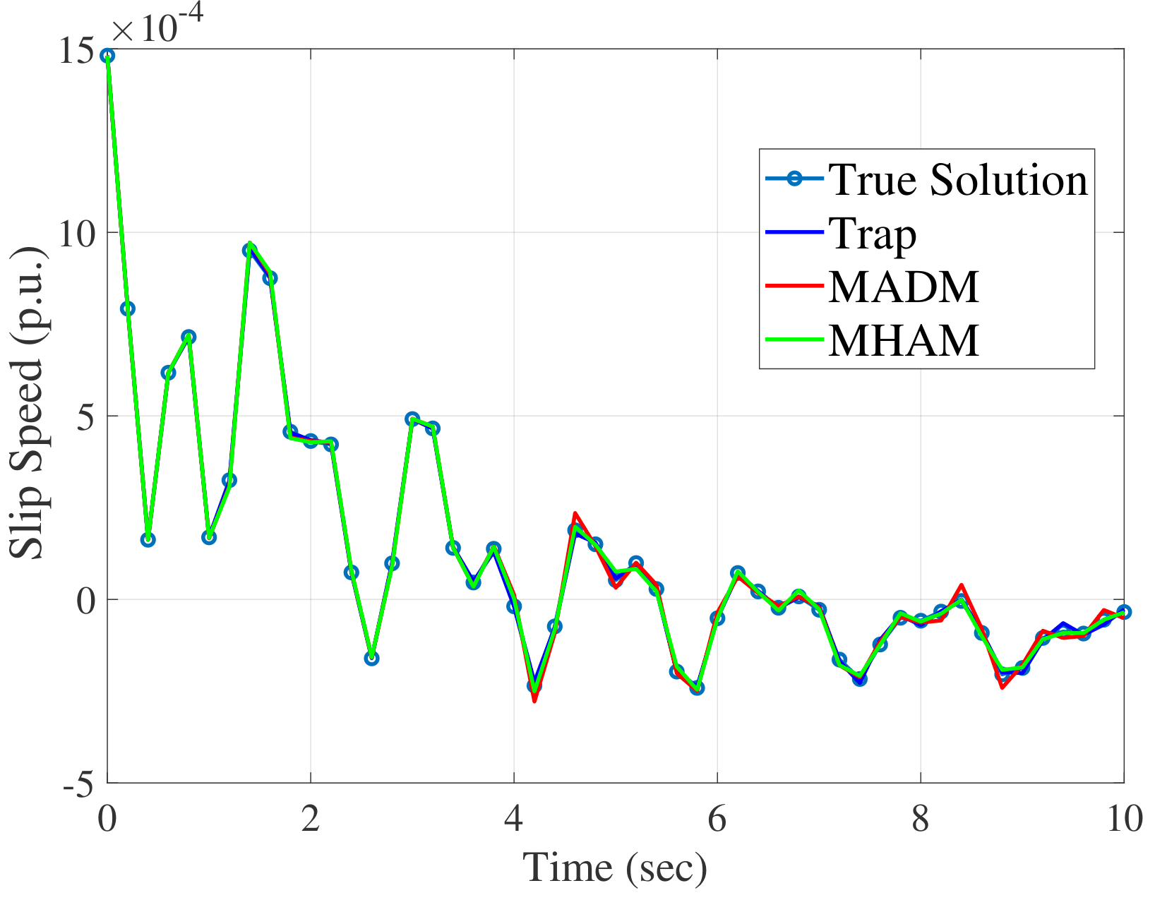
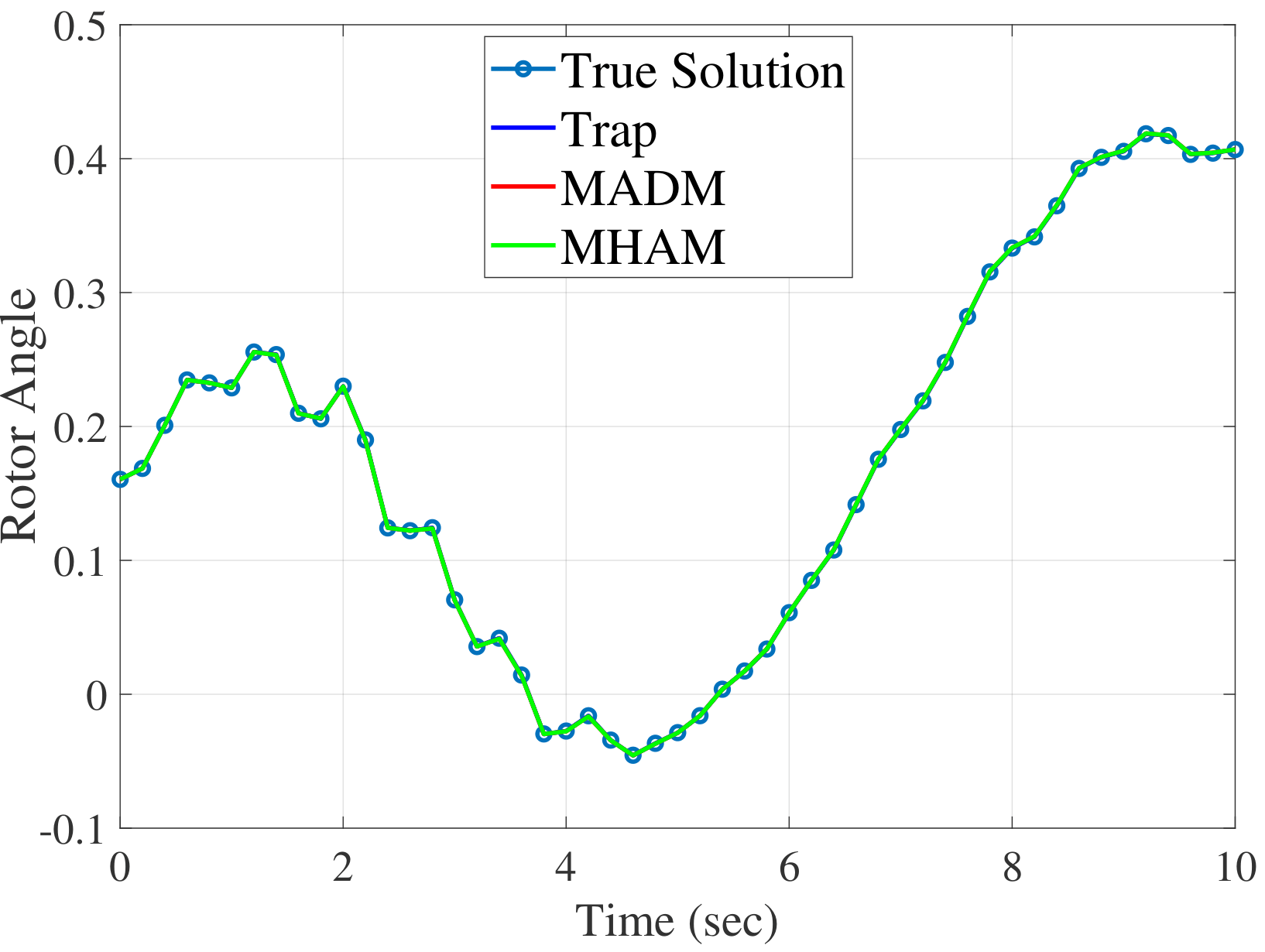
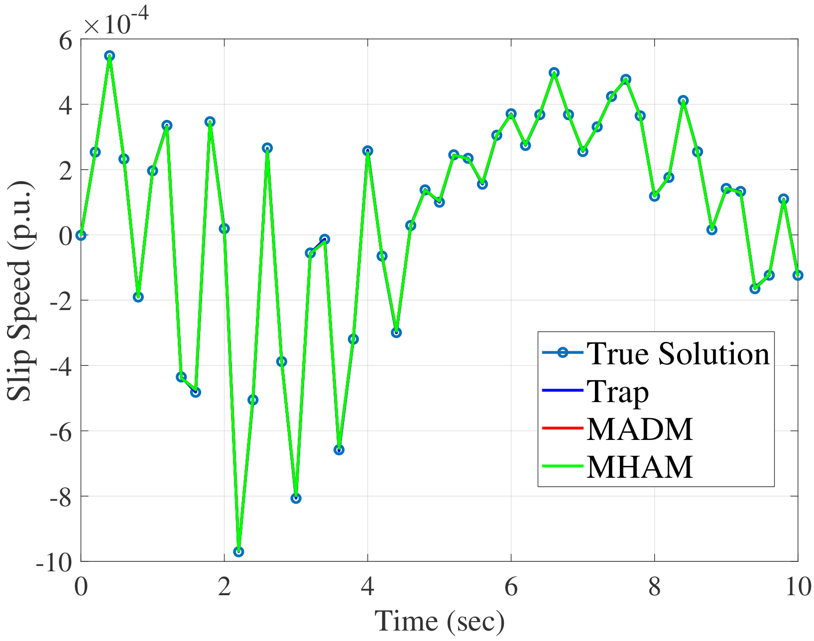
This section presents numerical case studies investigating the Parareal algorithm for power system dynamic simulations. We consider two test networks, the New England 10-generator 39-bus system [Pad02] as a small test network, and the Polish 327-generator 2383-bus system [ZMST11] as a large test network. Simulations are performed on Intel Core i7 2.59 GHz processors. The following disturbances are considered: 3-phase faults on buses with 4 cycles fault duration; 3-phase faults on branches with 4 cycles fault duration; and 3-phase faults on branches followed by tripping of that branch with 4 cycles fault duration. This section provides the representative result with the 3-phase fault at the bus 1 with 4 cycles since extensive numerical experiments showed a very similar pattern of simulation results across many disturbances.

Considering the allowable processors with a personal laptop in Python, the number of processors for parallel computing of the fine solver is chosen as 50. The 10$s$ simulation is conducted and thus divided into 50 sub-intervals. For each processor, 100 sub-intervals are used for the fine solver, indicating $\delta t=\frac{10}{50\times100}=0.002s$, but we vary the number of sub-intervals for the coarse operator.

Validation of Parareal Algorithm

Results with the New England 10-Generator 39-Bus System

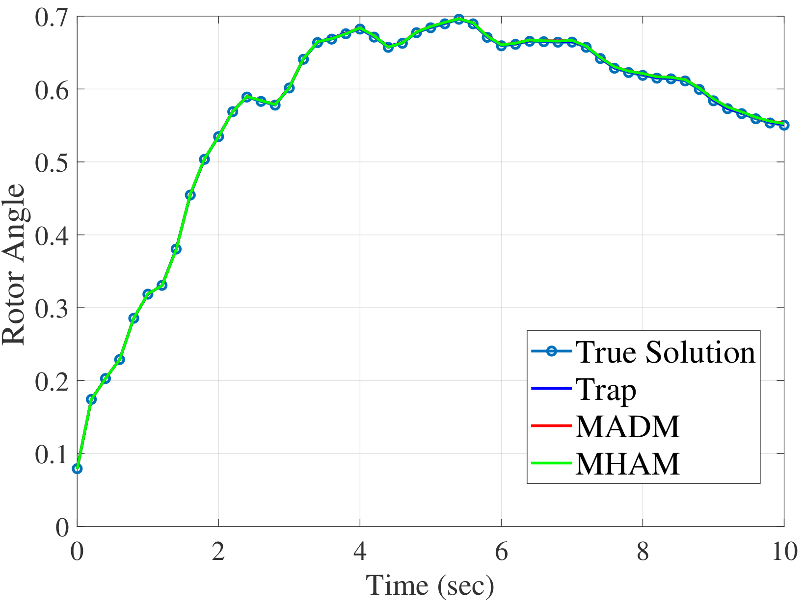
fig-nedelta-fig-neslip shows simulation results of Parareal algorithm for the $10s$ simulation with the New England system. This analysis uses 10 sub-intervals for the coarse operators in each processor, and the true solution is obtained using the standard sequential RK4 method with the time step of $0.002s$. The $m=3$ is used for the number of terms for both the MADM and MHAM. For the MAHM, $h=-0.9$ is used. As depicted, rotor angle and slip speed at bus 1 of the Parareal solution converged to the true solution with all three coarse operators. We have checked this convergence for other variables and disturbances to validate the convergence of Parareal algorithm.

Results with the Polish System, 327-Generator 2383-Bus

To further evaluate the performance of the Parareal algorithm, we have considered the large Polish system. The simulation setup is the same as the one used in Section 7.1.1. fig-pdelta-fig-pslip shows the convergence of Parareal algorithm for the $10s$ simulation. Similarly, we have also checked this convergence for other variables and disturbances to validate the convergence of Parareal algorithm for the Polish system.

Acknowledgments

The project was funded by the U.S. Department of Energy (DOE) Office of Electricity, Advanced Grid Research and Development Division. The authors acknowledge Dr. Ali Ghassemian from the DOE Office of Electricity for his continuing support and guidance.

Python Files and Functions

This appendix lists all of the python files and functions that the toolbox provides, except for those that are not required for a high level understanding of the toolbox. In most cases, the function is found in a python “py” file of the same name in the directory of the distribution.

Quick Start Guide

To get started, extract the zip archive of the python functions and IEEE testcases to a convenient place.

Soution Approach

para_real.py

Main python code to run the simulation using Parareal algorithm. As an example, the simulation can be run from the command line with following arguments.

mpiexec -n 50 python para_real.py 0 1 --nCoarse 10 --nFine 100 --tol 0.01 --tolcheck maxabs --debug 1 --fault fault.json --dist dist.json -o result.csv

This runs RAPID on 50 processors, which corresponds to 50 subintervals, with defined time increments (i.e., 10 time increments for the coarse operator in each of 50 subintervals and 100 time increments for the fine operator in each of 50 subintervals), using tolerance of 0.01 for maximum absolute value of the difference between iterations, reads fault scenarios defined in the fault.json file, includes the distribution network defined in the dist.json file, and then saves solutions into the result.csv file.

Function Descriptions

The function descriptions of this section are based on the python codes contained in the Parareal solution approach.

PowerModel.py

Read data and do post-processing (e.g., the calculation of initial conditions and define indices) before the simulation.
- makeYbus.py
  
  Construct the $Y_{bus}$ matrix.
- makeSbus.py
  
  Construct the complex bus power (Sbus) injecton vector
- newtonpf.py
  
  Run Newton Raphson to solve the power flow problem.
- pfsoln.py
  
  Organize the power flow solution.
pdefault.py

Using the “argparse” module, define command-line arguments.
packer.py

Pack or unpack variables.
Fault.py

Define the fault and modify the parameters accordingly for the post-fault simulation.
- fault.json
  
  The usage of the json module that the user can define faults in detail with many different attributes (e.g., fault type, start time, and end time) and interface with Python.
- ffault.py
  
  According to the fault type, modify the $Y_{bus}$ matrix and other parameters.
Coarse.py

Determine the solution method to be used for the coarse operator.
Fine.py

Determine the solution method to be used for the fine operator.
fn.py

Define the solution method.
- fnRK4
  
  The Runge-Kutta 4th order method.
- fnTrap
  
  The Midpoint-Trapezoidal predictor-corrector (Trap) method.
- fnTrap_adap
  
  The adaptive Trap method with approximate models by linearizing the underlying physics within relatively less important regions.
- fnADM
  
  The Adomian decomposition method.
- fnHAM
  
  The Homopoty analysis method.

Data

The toolbox takes as an input a MAT file written in the MATLAB language. Currently, these MAT files are loaded using the “loadmat” module from Scipy in the Python programming language.

Data_NE

The IEEE New England 10-generator 39-bus test network [Pad02] as a small-scale test network.
Data_POLISH

The IEEE Polish 327-generator 2383-bus system [ZMST11] as a large-scale test network.

SAS method options

The two SAS methods employed can adjust the number of SAS terms (and the auxiliary parameter $h$ for the HAM method) to affect the convergence rate (and region).

ADM method

The number of ADM terms can vary from 3 up to 10.
HAM method

The number of HAM terms is set to 3, but one can adjust the value of the auxiliary parameter $h$ to adjust the convergence region.

Optimal Homotopy Analysis Method

This section illustrates the potential upgrade to the standard HAM method. Notice that this approach is not extensively implemented in the current toolbox.

Notice that the original HAM provide an additional flexbility with the auxiliary parameter $h$ to adjust and control the convergence region and rate. This implies that one might seek to find an optimal value of $h$ to improve the performance of the original HAM. In this case, the optimal value of $h$ might be obtained by minimizing the squared residual error of governing equations. Let $R(h)$ denote the square residual error of the governing equation as follows:

\[\begin{aligned} R(h) = (N[x^{\text{HAM}}(t)])^2\end{aligned}\]

where $x^{\text{HAM}}(t)$ is a semi-analytical solution obtained from the HAM. Then, the optimal value of $h$ is given by solving the following nonlinear algebraic equation

\[\begin{aligned} \label{eq:OHAM1} \frac{dR(h)}{dh} = 0\end{aligned}\]

To obtain $h$ which satisfies [eq:OHAM1], the following assumptions are made

The auxiliary parameter $h$ is distributed to each device.
Each device is decoupled from other devices.
Consider up to 3 HAM terms.

The main reason is that one wishes [eq:OHAM1] to be a linear equation with only one $h$ variable so that one can just find an optimal $h$ without iterative methods. If one does not have one of these conditions, then it is not guaranteed. For example, without 2., [eq:OHAM1] can become nonlinear equation and can have $h$ whose power can be more than 2. Hence, it becomes complicated and $h$ can be a complex number. Also, without 1., [eq:OHAM1] becomes nonlinear equation, having $h$ from other devices.

With this setup, the following section describes the procedure to obtain an optimal $h$ for the turbine and governor as an example.

Turbine Model

\[\begin{split}\begin{aligned} \nonumber T_{m}^{HAM} & = T_{m,0} + T_{m,1} + T_{m,2} \\ \nonumber & = T_{m,0} + \pmb { h \Big[ + \frac{1}{T_{ch}}T_{m,0} - \frac{1}{T_{ch}}P_{sv,0} \Big] \Delta t } \\ & \quad + \pmb{ (1+h)T_{m,1} + h\frac{1}{2}\frac{1}{T_{ch}}T_{m,1}\Delta t} \\ \nonumber & = T_{m,0} + h\frac{1}{T_{ch}}T_{m,0}t - h\frac{1}{T_{ch}}P_{sv,0}t \\ & \quad + (1+h)h\frac{1}{T_{ch}}(T_{m,0}t - P_{sv,0}t) + h\frac{1}{2}\frac{1}{T_{ch}} h\frac{1}{T_{ch}} (T_{m,0}t - P_{sv,0}t)t \\ \nonumber & = T_{m,0} + ht\frac{1}{T_{ch}}(T_{m,0} - P_{sv,0} ) \\ \nonumber & \quad + ht\frac{1}{T_{ch}}(T_{m,0} - P_{sv,0} ) + h^2t\frac{1}{T_{ch}}(T_{m,0} - P_{sv,0}) \\ & \quad + h^2t^2\frac{1}{2}\frac{1}{T_{ch}^2} (T_{m,0} - P_{sv,0}) \end{aligned}\end{split}\]

Therefore,

\[\begin{split}\begin{aligned} \nonumber \dot{T}_{m}^{HAM} & = h\frac{1}{T_{ch}}(T_{m,0} - P_{sv,0} ) \\ \nonumber & \quad + h\frac{1}{T_{ch}}(T_{m,0} - P_{sv,0} ) + h^2\frac{1}{T_{ch}}(T_{m,0} - P_{sv,0}) \\ & \quad + h^2t\frac{1}{T_{ch}^2} (T_{m,0} - P_{sv,0})\end{aligned}\end{split}\]

Then, plug into $N(h)$.

\[\begin{aligned} N(h) = \dot{T}_{m}^{HAM} - \frac{1}{T_{ch}}(-T_m^{HAM} +P_{sv,0}) = 0\end{aligned}\]

Therefore,

\[\begin{split}\begin{aligned} \nonumber N(h) & = h\frac{1}{T_{ch}}(T_{m,0} - P_{sv,0} ) + h\frac{1}{T_{ch}}(T_{m,0} - P_{sv,0} ) + ... \\ & \quad + \frac{1}{T_{ch}} [T_{m,0} + ht\frac{1}{T_{ch}}(T_{m,0} - P_{sv,0} ) + ... - P_{sv,0}]\end{aligned}\end{split}\]

Then,

\[\begin{split}\begin{aligned} R(h) & = [N(h)]^2 \\ \frac{dR(h)}{dh} & = 2N(h)\frac{dN(h)}{dh}\end{aligned}\end{split}\]

To satisfy $\frac{dR(h)}{dh} = 0$, we need to have either $2N(h) = 0$ or $\frac{dN(h)}{dh} = 0.$ Since $N(h)$ is a quadratic function of $h$ which implies that $h$ can be a complex number, it is not our interest. So, we want $\frac{dN(h)}{dh} = 0.$

\[\begin{split}\begin{aligned} \nonumber \frac{dN(h)}{dh} & = \frac{1}{T_{ch}}(T_{m,0} - P_{sv,0}) + \frac{1}{T_{ch}}(T_{m,0} - P_{sv,0}) \\ \nonumber & \quad 2h\frac{1}{T_{ch}}(T_{m,0} - P_{sv,0}) + 2ht\frac{1}{T_{ch}^2} (T_{m,0} - P_{sv,0}) \\ \nonumber & \quad + \frac{1}{T_{ch}}\Big[t\frac{1}{T_{ch}}(T_{m,0} - P_{sv,0} ) + t\frac{1}{T_{ch}}(T_{m,0} - P_{sv,0} ) \\ & \quad + 2ht\frac{1}{T_{ch}}(T_{m,0} - P_{sv,0}) + ht^2\frac{1}{T_{ch}^2} (T_{m,0} - P_{sv,0}) - P_{sv,0} \Big] \\ & = (T_{m,0} - P_{sv,0}) \Big( 2\frac{1}{T_{ch}} + 2h\frac{1}{T_{ch}} + 2ht\frac{1}{T_{ch}^2} + 2\frac{1}{T_{ch}^2}t + 2ht\frac{1}{T_{ch}^2} + ht^2 \frac{1}{T_{ch}^3} \Big) \end{aligned}\end{split}\]

Then,

\[\begin{split}\begin{aligned} (T_{m,0} - P_{sv,0}) & \Big( 2\frac{1}{T_{ch}} + 2h\frac{1}{T_{ch}} + 2ht\frac{1}{T_{ch}^2} + 2\frac{1}{T_{ch}^2}t + 2ht\frac{1}{T_{ch}^2} + ht^2 \frac{1}{T_{ch}^3} \Big) = 0 \\ (T_{m,0} - P_{sv,0}) & \Big( h(2\frac{1}{T_{ch}} + 2t\frac{1}{T_{ch}^2} + 2t\frac{1}{T_{ch}^2} + t^2 \frac{1}{T_{ch}^3} ) + 2\frac{1}{T_{ch}} + 2\frac{1}{T_{ch}^2}t \Big) = 0 \\ (T_{m,0} - P_{sv,0})& h(2\frac{1}{T_{ch}} + 2t\frac{1}{T_{ch}^2} + 2t\frac{1}{T_{ch}^2} + t^2 \frac{1}{T_{ch}^3} ) = -(T_{m,0} - P_{sv,0})(2\frac{1}{T_{ch}} + 2\frac{1}{T_{ch}^2}t) \\ h & = \frac{-(T_{m,0} - P_{sv,0})(2\frac{1}{T_{ch}} + 2\frac{1}{T_{ch}^2}t) }{(T_{m,0} - P_{sv,0})(2\frac{1}{T_{ch}} + 2t\frac{1}{T_{ch}^2} + 2t\frac{1}{T_{ch}^2} + t^2 \frac{1}{T_{ch}^3} )}\end{aligned}\end{split}\]

Governor Model

\[\begin{split}\begin{aligned} \nonumber P_{sv}^{HAM} & = P_{sv,0} + P_{sv,1} + P_{sv,2} \\ \nonumber & = P_{sv,0} + \pmb { h \Big[ + \frac{1}{T_{sv}}P_{sv,0} - \frac{1}{T_{sv}} P_c + \frac{1}{T_{sv}} \frac{1}{R_D} \omega_{0} \Big] \Delta t } \\ & \quad + \pmb{ (1+h)P_{sv,1} + h\frac{1}{2}\frac{1}{T_{sv}}P_{sv,1}\Delta t } \\ \nonumber & = P_{sv,0} + h\frac{1}{T_{sv}}P_{sv,0}t - h\frac{1}{T_{sv}}P_{c}t + h\frac{1}{T_{sv}}\omega_{0}t \\ \nonumber & \quad + (1+h)h\frac{1}{T_{sv}}(P_{sv,0}t - P_ct + \frac{1}{R_D}\omega_{0}t) \\ & \quad + h\frac{1}{2}\frac{1}{T_{sv}} h\frac{1}{T_{sv}} (P_{sv,0}t - P_ct + \frac{1}{R_D}\omega_{0}t)t \\ \nonumber & = P_{sv,0} + h\frac{1}{T_{sv}}P_{sv,0}t - h\frac{1}{T_{sv}}P_{c}t + h\frac{1}{T_{sv}}\omega_{0}t \\ \nonumber & \quad + h\frac{1}{T_{sv}}P_{sv,0}t - h\frac{1}{T_{sv}}P_{c}t + h\frac{1}{T_{sv}}\frac{1}{R_D}\omega_{0}t \\ \nonumber & \quad + h^2\frac{1}{T_{sv}}P_{sv,0}t - h^2\frac{1}{T_{sv}}P_{c}t + h^2\frac{1}{T_{sv}}\frac{1}{R_D}\omega_{0}t \\ & \quad + h^2\frac{1}{2}\frac{1}{T_{sv}^2} P_{sv,0}t^2 - h^2\frac{1}{2}\frac{1}{T_{sv}^2} P_c t^2 + h^2\frac{1}{2}\frac{1}{T_{sv}^2} \frac{1}{R_D}\omega_{0}t^2\end{aligned}\end{split}\]

Table 1 Description of Sets
Set	Description
$\mathcal{N}$	Set of buses in the transmission network
$\mathcal{G}$	Set of generators in the transmission network
$\mathcal{I}$	Set of interfaces in the transmission network
$c \in \mathcal{C}$	Set of transmission connections in network
$t \in \mathcal{T}$	Set of time periods
$\mathcal{E} \subseteq \mat hcal{N} \times \mathcal{N} \times \mathcal{C}$	Set of lines in the transmission network
$\mathcal{E}_i \subseteq \m athcal{E}$	Subset of lines $\mathcal{E}$ belonging to interface $i \in \mathcal{I}$
$\mathcal{G}_i \in \mathcal {G}$	Subset of generators $\mathcal{G}$ at bus $i \in \mathcal{N}$

Aub11: Eric Aubanel. Scheduling of tasks in the parareal algorithm. Parallel Computing, 37(3):172–182, March 2011.
Dan03: P. L. Dandeno. IEEE guide for synchronous generator modeling practices and applications in power system stability analyses. IEEE Std. 1110-2002, pages 1–72, November 2003.
DG19(1,2): Disha Lagadamane Dinesha and Gurunath Gurrala. Application of multi-stage homotopy analysis method for power system dynamic simulations. IEEE Trans. Power Syst., 34(3):2251–2260, May 2019.
DRBW12: J. S. Duan, R. Rach, D. Baleanu, and A. M. Wazwaz. A review of the adomian decomposition method and its applications to fractional dierential equations. Commun. Fractional Calculus, 3(2):73–99, October 2012.
G+16(1,2): Gurunath Gurrala and others. Parareal in time for fast power system dynamic simulations. IEEE Trans. Power Syst., 31(3):1820–1830, May 2016.
G+17(1,2): Gurunath Gurrala and others. Large multi-machine power system simulations using multi-stage adomian decomposition. IEEE Trans. Power Syst., 32(5):3594–3606, September 2017.
KBL94: P. Kundur, N. Balu, and M. Lauby. Power System Stability and Control. McGraw-Hill, January 1994.
Lia09: S. Liao. Notes on the homotopy analysis method: some definitions and theorems. Commun. Nonlinear Sci. Numerical Simulation, 14(4):983–997, April 2009.
Lia03(1,2): Shijun Liao. Beyond Perturbation: Introduction to the Homotopy Analysis Method. Chapman and Hall/CRC, October 2003.
Pad02(1,2,3,4): K. R. Padiyar. Power System Dynamics Stability and Control. Hyderabad, India: B.S. Publications, 2002.
Pad08(1,2): K. R. Padiyar. Power System Dynamics: Stability & Control. BS Publications, 2008.
ZMST11(1,2,3): R. D. Zimmerman, C. E. Murillo-Sanchez, and R. J. Thomas. Matpower: steady-state operations, planning and analysis tools for power systems research and education. IEEE Trans. Power Syst., February 2011.

Set	Description
\(\mathcal{N}\)	Set of buses in the transmission network
\(\mathcal{G}\)	Set of generators in the transmission network
\(\mathcal{I}\)	Set of interfaces in the transmission network
\(c \in \mathcal{C}\)	Set of transmission connections in network
\(t \in \mathcal{T}\)	Set of time periods
\(\mathcal{E} \subseteq \mat hcal{N} \times \mathcal{N} \times \mathcal{C}\)	Set of lines in the transmission network
\(\mathcal{E}_i \subseteq \m athcal{E}\)	Subset of lines \(\mathcal{E}\) belonging to interface \(i \in \mathcal{I}\)
\(\mathcal{G}_i \in \mathcal {G}\)	Subset of generators \(\mathcal{G}\) at bus \(i \in \mathcal{N}\)

Welcome to RAPID’s documentation!

Installation

Citing \(RAPID\)

Collaboration

Data

Dynamic Data

Network Data

Modeling

Differential Equations

Synchronous Generator Model 2.2

Turbine Governor

IEEE Type-1 Excitation

Load Dynamic

Algebraic Equations

Stator Algebraic Equation

Network Algebraic Equation

Load Algebraic Equation

Dynamic Simulation

Initial Condition Calculations

Synchronous Generator Initial Conditions

Excitation System Initial Conditions

Governor Initial Conditions

Turbine Initial Conditions

Solution Approach

Parareal Algorithm

Parareal Implementation

Understanding of Parareal Algorithm

\(\textsf{para\_real.py}\)

Solution Method

Standard Numerical Iteration Method

Midpoint-Trapezoidal Predictor-Corrector

the Runge-Kutta 4th Order Method

Semi-Analytical Solution Method

Adomian Decomposition Method

The derivation of MADM terms for each device:

Homotopy Analysis Method

The derivation of MHAM terms for each device:

Summary

Simulation Results

Validation of Parareal Algorithm

Results with the New England 10-Generator 39-Bus System

Results with the Polish System, 327-Generator 2383-Bus

Acknowledgments

Python Files and Functions

Quick Start Guide

Soution Approach

Function Descriptions

Data

SAS method options

Optimal Homotopy Analysis Method

Turbine Model

Governor Model